Download
1 / 32
390 likes | 795 Views
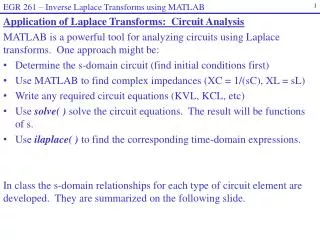
Introduction to Laplace Transforms. Def inition of the Laplace Transform. One-sided Laplace transform :. l Some functions may not have Laplace transforms but we do not use them in circuit analysis. Choose 0 - as the lower limit (to capture discontinuity in f(t) due to an event such as

E N D
Definition of the Laplace Transform One-sided Laplace transform: l Some functions may not have Laplace transforms but we do not use them incircuit analysis. Choose 0- as the lower limit (to capture discontinuity in f(t) due to an event such as closing a switch).
The sifting property: The impulse function is a derivative of the step function:
Laplace Transform Features 1) Multiplication by a constant 2) Addition (subtraction) 3) Differentiation
Laplace Transform Features (cont.) 3) Differentiation
Laplace Transform Features (cont.) 4) Integration 5) Translation in the Time Domain
Laplace Transform Features (cont.) 6) Translation in the Frequency Domain 7) Scale Changing
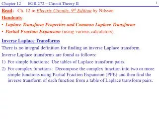
Partial Fraction Expansion Step1: Expand F(s) as a sum of partial fractions. Step 2: Compute the expansion constants (four cases) Step 3: Write the inverse transform
Whenever F(s) contains distinct complex roots at the denominator as (s+-j)(s++j), a pair of terms of the form appears in the partial fraction. Where K is a complex number in polar form K=|K|ej=|K| 0 and K* is the complex conjugate of K. The inverse Laplace transform of the complex-conjugate pair is
Improper Transfer Functions An improper transfer function can always be expanded into a polynomial plus a proper transfer function.
POLES AND ZEROS OF F(s) The rational function F(s) may be expressed as the ratio of two factored polynomials as The roots of the denominator polynomial –p1, -p2, ..., -pm are called the poles of F(s). At these values of s, F(s) becomes infinitely large. The roots of the numerator polynomial -z1, -z2, ..., -zn are called the zeros of F(s). At these values of s, F(s) becomes zero.
The poles of F(s) are at 0, -10, -6+j8, and –6-j8. The zeros of F(s) are at –5, -3+j4, -3-j4 num=conv([1 5],[1 6 25]); den=conv([1 10 0],[1 12 100]); pzmap(num,den)
Initial-Value Theorem The initial-value theorem enables us to determine the value of f(t) at t=0 from F(s). This theorem assumes that f(t) contains no impulse functions and poles of F(s), except for a first-order pole at the origin, lie in the left half of the s plane.
Final-Value Theorem The final-value theorem enables us to determine the behavior of f(t) at infinity using F(s). The final-value theorem is useful only if f(∞) exists. This condition is true only if all the poles of F(s), except for a simple pole at the origin, lie in the left half of the s plane.