Download
1 / 35
490 likes | 1.17k Views
Lecture 4 Laplace Transforms and the Transfer Function. Advantages of Laplace Transforms. Standard notation in dynamics and control Converts mathematical operations into algebra Provides major insight by using block diagrams S traight-forward technique in control design

E N D
Advantages of Laplace Transforms • Standard notation in dynamics and control • Converts mathematical operations into algebra • Provides major insight by using block diagrams • Straight-forward technique in control design >>> leads to frequency response (steady-state)
Laplace Transforms Method to transform time scale (t) into a complex domain (s). Examples: Usually f(0) is set to 0, i.e., the error at time t= 0 is zero or steady state conditions exist.
Laplace Transforms in Process Control Laplace transforms are used in process control for several types of studies: • To solve linear differential equations • To analyze linear control systems • To predict transient response for different inputs • To determine frequency response of a system
28. Proportional Control Kcε(t)KcE(s) Integral Control E(s)/TIs Derivative Control TD sE(s)
The method can be used on any order of an ordinary differential equation, limited only by the factoring of the denominator polynomial (i.e., the characteristic equation). The procedure must be modified for equal roots and imaginary roots.
Useful feature of this approach is that the denominator of the transfer function can be studied directly to determine its poles or roots A pole = the reciprocal of a time constant. A root provides information about the exponential exponent in the time domain For example: The denominator can be factored into (2s + 1)(s+1) to give: From the two factors, we know that τ1 = ½ and τ2 = 1. However should the function be changed to:
This system must be unstable. It will have a transient response (to a step change) that includes the following terms: e½t and e-t Obviously the former term is unbounded as t increases. In analyzing the stability of a control system, the exponent of all exponentials must be negative in order for the system to reach a new steady-state value.
First Order System Y(s) = G(s) U(s) G(s) is called a system transfer function. It is an intrinsic property of the system independent of input changes.
Second Order System So there are three possible solutions which depend on the value of ζ ζ> 1 Overdamped ζ= 1 Critically damped ζ< 1 Underdamped
Block Diagram Algebra and Notation Consider the Transfer Function G(s): composed of two first order subsystems G1(s) and G2(s): (a) Multiplicative rule (b) Additive rule
Equivalent Systems Asystem with a measurement block can be replaced with an "equivalent" single block system by finding the overall system transfer function by developing equations for the new system so the control and error ratios are identical:
Forcing Functions Once a dynamic model has been created, the next step is to study its response to input variable changes. In conducting these studies, one input is varied according to some specific function while the other variables are held constant. These disturbances are known as "forcing functions" since their role is to "force" a known change within the control system. There are four basic types of forcing functions: - step change (transient response) - ramp change (used to establish models for uncontrollable variables) - sine wave change (frequency response – steady-state response) - impulse change (used to determine residence time)
Response to an Impulse Function The system (or process) response to an impulse change depends on the degree of mixing in the process. If the model operates according to plug flow (first-in/first-out) then the output will be as follows: • Plug Flow would be typical of a large TD value relative to a short or zero Tp value • - Mixed Flow would be typical of a short or zero TD value relative to the Tpvalue Should the process operate as a fully-mixed system, then the output will be:
Response to an Impulse Function In reality, the real response will lie somewhere between these two extremes. The time delay consists of a pure delay component and a distributed component. The response to an impulse change for a series of tanks is shown below. The variable "n" is the number of fully-mixed tanks. As the number increases, the overall response approaches plug-flow. tR = V/Q