Download
1 / 36
420 likes | 1.8k Views
Waiting Line Models ( Queuing Theory). Examples of Lines in Operations Management. Assembly lines Production lines Trucks waiting to unload or load Workers waiting for parts Customers waiting for products Broken equipment waiting to be fixed Customers waiting for service.

E N D
Waiting Line Models (Queuing Theory)
Examples of Lines in Operations Management • Assembly lines • Production lines • Trucks waiting to unload or load • Workers waiting for parts • Customers waiting for products • Broken equipment waiting to be fixed • Customers waiting for service
Why We Analyze Waiting Lines • Lines cost a business money. • The resources in a line (people and/or material) are idle and thus unproductive. • The resources needed to process/service a line (cashiers, dock workers, equipment, etc.) cost a business money. • There is an ideal length for a line that minimizes the total cost of the line. • No line is wasteful of the resources being used to process lines.
Costs • The costs of waiting in line • Paying idle employees while they are in line waiting for something they need. (waiting for parts, supplies, etc.) • Unusable equipment awaiting repairs • EG: Broken assembly line machinery. • Losing customers because of long lines • Reneging: Customers get tired of waiting and leave • Balking: Customers see a long line and don’t get in line. • The cost of providing service to the line • Paying people who are servicing the customers. • Customers can be people, machines, or other objects needing service.
Examples of The Cost of Providing Service • Paying repairmen to fix broken machines • Paying dock workers to load and unload trucks • Paying customer-service people • Using extra production people to speed up a line • Leasing service equipment and facilities • Paying checkout cashiers
Total Cost Cost of Servicegoes up as you pay for more servers. Costs of Waitinggoes down as more servers reduce the # of customers in line. Optimal # of servers Queuing System Costs Costs Fewer servers often means longer waiting for customers. Many servers means little or no waiting, but higher service costs. Number of Servers Note that the lowest cost system requires some customer waiting.
What Queuing Models Tell Us. • Average number of customers in line. • Averagetime in line for a customer. • Average number of customers in the system at any time. (In line and being served.) • Averagetime in the system for a customer. • Probabilityof n number of customers in the system at any given time. • NOTE: “In The System” includes customers who are waiting plus and the customers being served.
ARRIVAL SYSTEM(How customers arrive) QUEUE(The nature of the waiting line or lines of customers) The Waiting Line System SERVICE FACILITY (How customers progress through a service facility)
Customer population Service System Waiting line (Queue) Served customers Service facilities Priority rule Waiting Line Models Arrival System The sequence in which customers are admitted into the service facility.
Arrival System • Arrival Populations are either… • Limited (EG: Only people age 21 or over.) • Unlimited (EG: cars arriving at a toll booth) • Arrival Patterns are either… • Random (Each arrival is independent) • Scheduled (EG: Doctor’s office visits) • Behavior of the Arrivals • Balking (Seeing a long line and avoiding it.) • Reneging (Get tired of waiting and leave the line) • Jockeying (Switching lines)
The Queue (line) • Queue Length (line length) is either.. • Unlimited (EG: cars in line at a toll booth) • Limited (Finite) EG: # of e-mail messages allowed. • Queue Discipline (order of service) • FIFO (First-In, First-Out) • LIFO (Last-In, First-Out) • SIRO (Service In Random Order) • Priority
The Service Facility • Channels are the paths (ways to get through the system) after getting in line? • EG: McDonalds drive-thru is one channel. • Phases are the number of stops a customer must make, after getting in line? (Single-phase means only one stop for service.) • McDonalds drive-thru is a single-channel, three-phase system:OrderPayPick-up
Single-channel, Single-phaseOne way through the system and one stop for service Service Facility
Multi-channel, Single-phase Once in line, you have two or more choices of how to get through the system, but only one stop. Service Facility Service Facility
Multi-channel, Multi-phase Once in line, you have at least two choices (channels) of how to get through the system and at least two stops (phases). Service Facility Service Facility Service Facility Service Facility
Four Single-channel, Single-phase Systems(Once in line, you only have one channel and one stop.) Service Facility Service Facility Service Facility Service Facility
One, Multi-channel, Single-Phase System (Once in line you have four possible paths through the system, but only one stop.) Service Facility Service Facility Service Facility Service Facility
Assumptions We Will Use • The Rate of Service must be faster than the Rate of Arrivals. (It is unsolvable if customers arrive faster than they can be served.) • Always enter the service rate for 1 server. The model will compute the total service rate based on the number of servers. • FIFO (First In, First Out) (Customers are served in the order they arrive.) • Arrivals are unlimited (infinite) • Arrivals are random rather than scheduled. • Customers arrive independently of each other. • Service times can vary from one customer to another, and are independent of each other. (Customers may have different service needs and times.)
Queuing Problem At a large Naval Ship Repair Facility mechanics have to make frequent trips to the tool crib for parts and specialized equipment. Arrivals are infinite (unrestricted) since mechanics can come as often as need, even though the population of customers is finite.) Records indicate that the tool crib servesan average of 18 mechanics each hour, but one attendant is capable of serving 20 per hour. If mechanics are paid $30 per hour and the tool crib attendants make $9 per hour, would it be more cost effective to have one or two attendants in the tool crib? The service rate is always the average rate for one server, regardless of how many servers there are in the system. In this case the service rate of 20 is higher than the arrival rate of 18. If the service rate had been 10 customers per server, you would need to enter at least two servers or the model would not have worked.
Which system is less expensive? Single Attendant 1st Attendant 2nd Attendant (It depends on the cost of service versus the cost of waiting.)
Data-Entry Information for POM/QM One attendant can serve 20mechanics/customers per hr. and is paid $9 per hour. $9/hr Single Attendant $30/hr Mechanics (customers) arrive at an average of 18 per hourand are paid $30 per hour. 1st Attendant 2nd Attendant I ran the POM-QM model using two servers, but I could have run it with any number of servers since you alwaysenter the service rate for one server. The POM-QM model will do the computations for more than one server.
Select the Module Select the M/M/s Model
Make sure you use the M/M model. Results for 2 servers • Average # customers in the system • Average time spent in the system • Average time spent in line • Average # of customers in line
Find the optimal # of servers Lowest Cost is $51.86 when using two servers. • In this problem, you would have gotten this screen regardless of how many servers you used for the input, because the service rate for one server exceeded the arrival rate. • The single-server rate times the number of servers you enter must exceed the arrival rate. If the single-server rate in this problem had been 6 per hour instead of 20 per hour, you would have had to enter at least 4 servers. (Three servers would have served 18 per hour, which does not exceed the arrival rate of 18.)
The probability that 4 or fewer mechanics are in the system is 97% Probability that the system is idle (no customers) is 38%
Average # customers in the system Average time in the system (min.) Average # customers in line Average time in line (min.) Probability that the system is idle 9 1.13 30 3.76 8.1 0.23 270.76 10%38% # of Servers 1 2 What the Model Tells Us… Note: You need to run the model with 1 server if you want the info for 1 server, and run it using 2 servers to get the info for 2 servers. Once you know the optimal # of servers, make sure you run it again for that many servers in order to get the right data. But always enter the service rate for one server, regardless of how many servers.
POM/QM or Excel Solver? POM/QM will do the cost analysis for you, so it is easier. (Select the “M/M” model.) You can use the Excel Solver, but it won’t do the cost analysis, so you would need to do that manually. You also need to run the Excel Solver once for each server number you use, and then do a manual cost analysis for each in order to see which number of servers has the lowest cost. In multiple server problems, you might have to run the Solver for a half-dozen or more scenarios.
Manual cost computations for one server (9 customers in the system) • Mechanics get paid $30 per hour Cost of waiting is: $30 x 9customers in system = $270 • Attendantsget paid $9 per hour Cost of service is thus 1 server x $9 = $9 per hour • System cost with one server is: $270 + $9 = $279 POM-QM model
Manual cost computations for Two servers (9 customers in the system) • Mechanics get paid $30 per hour Cost of waiting is: $30 x 1.28 customers in system = $33.84 • Attendantsget paid $9 per hour Cost of service is: $9 x2 servers = $18 per hour • Total cost with two servers is: $18 + $33.84 = $51.84 POM-QM model
Homework Assignment Due next Tuesday Problem 1: Auto Repair Center Problem 2: The Quarry Use POM/OM or Excel Solver software and submit printouts to support your decisions
Car Repair In the service department of a repair shop, mechanics requiring parts for repair or service present their request forms at the parts department counter. The parts clerk fills a request while the mechanic waits. Mechanics arrive in a random fashion at the rate of 35 per hour, and a clerk can fill requests at the rate of 20 per hour. If the cost for a parts clerk is $12 per hour and the cost for a mechanic is $25 per hour, determine the optimum number of clerks to staff the counter. (Because of the high arrival rate, an infinite source may be assumed.) Always enter the service rate for one server. The program will do the math once you enter the number of servers. If you enter fewer servers than can handle the arrival needs, the program will give you an error message because the computed service rate must be higher than the arrival rate.
The Quarry (no cost analysis in model) You are in charge of a quarry that supplies sand and stone aggregates to construction sites. Empty trucks arrive and wait in line for loading either sand or aggregate. At the loading station they are filled with material, weighted, checked out, and then proceed to a construction site. Currently9 empty trucks arrive each hour (on average) In addition to waiting in line, it takes 6 minutes for a truck to be filled, weighed and checked out. (Only one loading station is available.)Concerned that trucks are spending too much time waiting and being filled, you evaluate the current situationand compare it to each alternative below. Alternative 1: Speed up the loading process and add side boards to the trucks so that more material can be loaded faster. This will improve the speed of loading, but cost $50,000. Since the trucks hold more, their arrival rate would be reduced to 6 per hour and loading time becomes 15 an hour. Alternative 2: Add a second loading station at a cost of $80,000. The trucks would arrive at the current rate of 9 per hour. They would then wait in a common line and the truck at the front of the line would move to the next available loading station. Loading time at each of the stations is 6 minutes. Which alternative do you recommend? (Select “No Cost” in the POM/QM waiting line model. You must decide which of the three situations would the most cost-effective based on time in the system and upgrade costs.