Download
1 / 84
870 likes | 1.11k Views
8. Economic Growth II: Technology, Empirics, and Policy. Introduction. In the Solow model of Chapter 7, the production technology is held constant. income per capita is constant in the steady state. Neither point is true in the real world:

E N D
8 Economic Growth II:Technology, Empirics, and Policy
Introduction In the Solow model of Chapter 7, • the production technology is held constant. • income per capita is constant in the steady state. Neither point is true in the real world: • 1904-2004: U.S. real GDP per person grew by a factor of 7.6, or 2% per year. • examples of technological progress abound(see next slide). CHAPTER 8 Economic Growth II
Technological progress in the Solow model • A new variable: E = labor efficiency • Assume: Technological progress is labor-augmenting: it increases labor efficiency at the exogenous rate g: CHAPTER 8 Economic Growth II
Technological progress in the Solow model • We now write the production function as: • where LE = the number of effective workers. • Increases in labor efficiency have the same effect on output as increases in the labor force. CHAPTER 8 Economic Growth II
Technological progress in the Solow model • Notation: y = Y/LE = output per effective worker k = K/LE = capital per effective worker • Production function per effective worker:y = f(k) • Saving and investment per effective worker:sy = sf(k) CHAPTER 8 Economic Growth II
Technological progress in the Solow model ( +n +g)k = break-even investment: the amount of investment necessary to keep k constant. Consists of: • k to replace depreciating capital • nk to provide capital for new workers • gk to provide capital for the new “effective” workers created by technological progress CHAPTER 8 Economic Growth II
Investment, break-even investment (+n+g)k sf(k) k* Capital per worker, k Technological progress in the Solow model k=s f(k) ( +n +g)k CHAPTER 8 Economic Growth II
Variable Symbol Steady-state growth rate Steady-state growth rates in the Solow model with tech. progress Capital per effective worker k =K/(LE ) 0 Output per effective worker y =Y/(LE ) 0 Output per worker (Y/L) = yE g Total output Y = yEL n + g CHAPTER 8 Economic Growth II
The Golden Rule To find the Golden Rule capital stock, express c* in terms of k*: c* = y*i* = f(k*) ( +n +g)k* c* is maximized when MPK = +n+g or equivalently, MPK = n+g In the Golden Rule steady state, the marginal product of capital net of depreciation equals the pop. growth rate plus the rate of tech progress. CHAPTER 8 Economic Growth II
Growth empirics: Balanced growth • Solow model’s steady state exhibits balanced growth - many variables grow at the same rate. • Solow model predicts Y/L and K/L grow at the same rate (g), so K/Y should be constant. • This is true in the real world. • Solow model predicts real wage grows at same rate as Y/L, while real rental price is constant. • This is also true in the real world. CHAPTER 8 Economic Growth II
Growth empirics: Convergence • Solow model predicts that, other things equal, “poor” countries (with lower Y/L and K/L) should grow faster than “rich” ones. • If true, then the income gap between rich & poor countries would shrink over time, causing living standards to “converge.” • In real world, many poor countries do NOT grow faster than rich ones. Does this mean the Solow model fails? CHAPTER 8 Economic Growth II
Growth Empirics: Convergence • Solow model predicts that, other things equal, “poor” countries (with lower Y/L and K/L) should grow faster than “rich” ones. • No, because “other things” aren’t equal. • In samples of countries with similar savings & pop. growth rates, income gaps shrink about 2% per year. • In larger samples, after controlling for differences in saving, pop. growth, and human capital, incomes converge by about 2% per year. CHAPTER 8 Economic Growth II
Growth empirics: Convergence • What the Solow model really predicts is conditional convergence - countries converge to their own steady states, which are determined by saving, population growth, and education. • This prediction comes true in the real world. CHAPTER 8 Economic Growth II
Growth empirics: Factor accumulation vs. production efficiency • Differences in income per capita among countries can be due to differences in 1. capital – physical or human – per worker 2. the efficiency of production (the height of the production function) • Studies: • both factors are important. • the two factors are correlated: countries with higher physical or human capital per worker also tend to have higher production efficiency. CHAPTER 8 Economic Growth II
Growth empirics: Factor accumulation vs. production efficiency • Possible explanations for the correlation between capital per worker and production efficiency: • Production efficiency encourages capital accumulation. • Capital accumulation has externalities that raise efficiency. • A third, unknown variable causes capital accumulation and efficiency to be higher in some countries than others. CHAPTER 8 Economic Growth II
Policy issues: Evaluating the rate of saving To estimate (MPK ), use three facts about the U.S. economy: 1. k = 2.5 yThe capital stock is about 2.5 times one year’s GDP. 2. k = 0.1 yAbout 10% of GDP is used to replace depreciating capital. 3. MPKk = 0.3 yCapital income is about 30% of GDP. CHAPTER 8 Economic Growth II
Policy issues: Evaluating the rate of saving 1. k = 2.5 y 2. k = 0.1 y 3. MPKk = 0.3 y To determine , divide 2 by 1: CHAPTER 8 Economic Growth II
Policy issues: Evaluating the rate of saving 1. k = 2.5 y 2. k = 0.1 y 3. MPKk = 0.3 y To determine MPK, divide 3 by 1: Hence, MPK = 0.12 0.04 = 0.08 CHAPTER 8 Economic Growth II
Policy issues: Evaluating the rate of saving • From the last slide: MPK = 0.08 • U.S. real GDP grows an average of 3% per year, so n+g = 0.03 • Thus, MPK = 0.08 > 0.03 = n+g • Conclusion: The U.S. is below the Golden Rule steady state: Increasing the U.S. saving rate would increase consumption per capita in the long run. CHAPTER 8 Economic Growth II
Policy issues: How to increase the saving rate • Reduce the government budget deficit(or increase the budget surplus). • Increase incentives for private saving: • reduce capital gains tax, corporate income tax, estate tax as they discourage saving. • replace federal income tax with a consumption tax. • expand tax incentives for IRAs (individual retirement accounts) and other retirement savings accounts. CHAPTER 8 Economic Growth II
Policy issues: Allocating the economy’s investment • In the Solow model, there’s one type of capital. • In the real world, there are many types,which we can divide into three categories: • private capital stock • public infrastructure • human capital: the knowledge and skills that workers acquire through education. • How should we allocate investment among these types? CHAPTER 8 Economic Growth II
Policy issues: Allocating the economy’s investment Two viewpoints: 1. Equalize tax treatment of all types of capital in all industries, then let the market allocate investment to the type with the highest marginal product. 2. Industrial policy: Govt should actively encourage investment in capital of certain types or in certain industries, because they may have positive externalities that private investors don’t consider. CHAPTER 8 Economic Growth II
Policy issues: Establishing the right institutions • Creating the right institutions is important for ensuring that resources are allocated to their best use. Examples: • Legal institutions, to protect property rights. • Capital markets, to help financial capital flow to the best investment projects. • A corruption-free government, to promote competition, enforce contracts, etc. CHAPTER 8 Economic Growth II
Growth in output per person (percent per year) Canada 2.9 1.8 France 4.3 1.6 Germany 5.7 2.0 Italy 4.9 2.3 Japan 8.2 2.6 U.K. 2.4 1.8 U.S. 2.2 1.5 CASE STUDY: The productivity slowdown 1948-72 1972-95 CHAPTER 8 Economic Growth II
Growth in output per person (percent per year) Canada 2.9 1.8 2.4 France 4.3 1.6 1.7 Germany 5.7 2.0 1.2 Italy 4.9 2.3 1.5 Japan 8.2 2.6 1.2 U.K. 2.4 1.8 2.5 U.S. 2.2 1.5 2.2 CASE STUDY: I.T. and the “New Economy” 1948-72 1972-95 1995-2004 CHAPTER 8 Economic Growth II
CASE STUDY: I.T. and the “New Economy” Apparently, the computer revolution did not affect aggregate productivity until the mid-1990s. Two reasons: 1. Computer industry’s share of GDP much bigger in late 1990s than earlier. 2. Takes time for firms to determine how to utilize new technology most effectively. The big, open question: • How long will I.T. remain an engine of growth? CHAPTER 8 Economic Growth II
Endogenous growth theory • Solow model: • sustained growth in living standards is due to tech progress. • the rate of tech progress is exogenous. • Endogenous growth theory: • a set of models in which the growth rate of productivity and living standards is endogenous. CHAPTER 8 Economic Growth II
A basic model • Production function: Y = AKwhere A is the amount of output for each unit of capital (A is exogenous & constant) • Key difference between this model & Solow: MPK is constant here, diminishes in Solow • Investment: sY • Depreciation: K • Equation of motion for total capital: K = sY K CHAPTER 8 Economic Growth II
A basic model K = sY K • Divide through by K and use Y = AK to get: • If sA > , then income will grow forever, and investment is the “engine of growth.” • Here, the permanent growth rate depends on s. In Solow model, it does not. CHAPTER 8 Economic Growth II
Does capital have diminishing returns or not? • Depends on definition of “capital.” • If “capital” is narrowly defined (only plant & equipment), then yes. • Advocates of endogenous growth theory argue that knowledge is a type of capital. • If so, then constant returns to capital is more plausible, and this model may be a good description of economic growth. CHAPTER 8 Economic Growth II
A two-sector model • Two sectors: • manufacturing firms produce goods. • research universities produce knowledge that increases labor efficiency in manufacturing. • u = fraction of labor in research (u is exogenous) • Mfg prod func: Y = F [K, (1-u)EL] • Res prod func: E = g(u)E • Cap accumulation: K = sY K CHAPTER 8 Economic Growth II
A two-sector model • In the steady state, mfg output per worker and the standard of living grow at rate E/E = g(u). • Key variables: s: affects the level of income, but not its growth rate (same as in Solow model) u: affects level and growth rate of income • Question: Would an increase in u be unambiguously good for the economy? CHAPTER 8 Economic Growth II
Facts about R&D 1. Much research is done by firms seeking profits. 2. Firms profit from research: • Patents create a stream of monopoly profits. • Extra profit from being first on the market with a new product. 3. Innovation produces externalities that reduce the cost of subsequent innovation. Much of the new endogenous growth theory attempts to incorporate these facts into models to better understand technological progress. CHAPTER 8 Economic Growth II
Chapter Summary 1. Key results fromSolow model with tech progress • steady state growth rate of income per person depends solely on the exogenous rate of tech progress • the U.S. has much less capital than the Golden Rule steady state 2. Ways to increase the saving rate • increase public saving (reduce budget deficit) • tax incentives for private saving CHAPTER 8 Economic Growth II slide 33
Chapter Summary 3. Productivity slowdown & “new economy” • Early 1970s: productivity growth fell in the U.S. and other countries. • Mid 1990s: productivity growth increased, probably because of advances in I.T. 4. Empirical studies • Solow model explains balanced growth, conditional convergence • Cross-country variation in living standards isdue to differences in cap. accumulation and in production efficiency CHAPTER 8 Economic Growth II slide 34
Chapter Summary 5. Endogenous growth theory: Models that • examine the determinants of the rate of tech. progress, which Solow takes as given. • explain decisions that determine the creation of knowledge through R&D. CHAPTER 8 Economic Growth II slide 35
9 Introduction to Economic Fluctuations
In this chapter, you will learn… • facts about the business cycle • how the short run differs from the long run • an introduction to aggregate demand • an introduction to aggregate supply in the short run and long run • how the model of aggregate demand and aggregate supply can be used to analyze the short-run and long-run effects of “shocks.” CHAPTER 8 Economic Growth II
Facts about the business cycle • GDP growth averages 3–3.5 percent per year over the long run with large fluctuations in the short run. • Consumption and investment fluctuate with GDP, but consumption tends to be less volatile and investment more volatile than GDP. • Unemployment rises during recessions and falls during expansions. • Okun’s Law: the negative relationship between GDP and unemployment. CHAPTER 8 Economic Growth II
Real GDP growth rate Consumption growth rate Average growth rate Growth rates of real GDP, consumption 10 Percent change from 4 quarters earlier 8 6 4 2 0 -2 -4 1970 1975 1980 1985 1990 1995 2000 2005 CHAPTER 8 Economic Growth II
Real GDP growth rate Investment growth rate Consumption growth rate Growth rates of real GDP, consumption, investment Percent change from 4 quarters earlier 40 30 20 10 0 -10 -20 -30 1970 1975 1980 1985 1990 1995 2000 2005 CHAPTER 8 Economic Growth II
1970 1975 1980 1985 1990 1995 2000 2005 Unemployment Percent of labor force 12 10 8 6 4 2 0 CHAPTER 8 Economic Growth II
1966 1951 1984 2003 1987 1975 2001 1982 1991 -3 -2 -1 0 1 2 3 4 Okun’s Law 10 Percentage change in real GDP 8 6 4 2 0 -2 -4 Change in unemployment rate CHAPTER 8 Economic Growth II
Index of Leading Economic Indicators • Published monthly by the Conference Board. • Aims to forecast changes in economic activity 6-9 months into the future. • Used in planning by businesses and govt, despite not being a perfect predictor. CHAPTER 8 Economic Growth II
Components of the LEI index • Average workweek in manufacturing • Initial weekly claims for unemployment insurance • New orders for consumer goods and materials • New orders, nondefense capital goods • Vendor performance • New building permits issued • Index of stock prices • M2 • Yield spread (10-year minus 3-month) on Treasuries • Index of consumer expectations CHAPTER 8 Economic Growth II
Index of Leading Economic Indicators 160 140 120 100 1996 = 100 80 60 40 20 0 Source: Conference Board 1970 1975 1980 1985 1990 1995 2000 2005 CHAPTER 8 Economic Growth II
Time horizons in macroeconomics • Long run: Prices are flexible, respond to changes in supply or demand. • Short run:Many prices are “sticky” at some predetermined level. The economy behaves much differently when prices are sticky. CHAPTER 8 Economic Growth II
Recap of classical macro theory (Chaps. 3-8) • Output is determined by the supply side: • supplies of capital, labor • technology. • Changes in demand for goods & services (C, I, G ) only affect prices, not quantities. • Assumes complete price flexibility. • Applies to the long run. CHAPTER 8 Economic Growth II
When prices are sticky… …output and employment also depend on demand, which is affected by • fiscal policy (G and T ) • monetary policy (M ) • other factors, like exogenous changes in C or I. CHAPTER 8 Economic Growth II
The Quantity Equation as Aggregate Demand • From Chapter 4, recall the quantity equation M V = P Y • For given values of M and V, this equation implies an inverse relationship between P and Y: CHAPTER 8 Economic Growth II