Verification for Hypersonic, Reacting Turbulent Flow

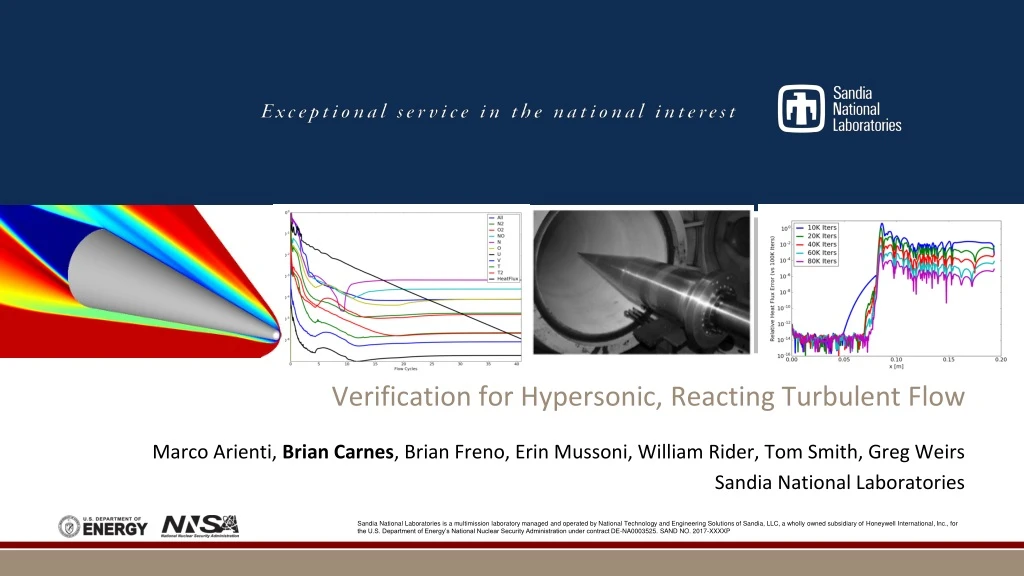
1. Verification for Hypersonic, Reacting Turbulent Flow Marco Arienti, Brian Carnes, Brian Freno, Erin Mussoni, William Rider, Tom Smith, Greg Weirs Sandia National Laboratories

2. Hypersonic Reentry Simulation Using SPARC • State-of-the-art hypersonic CFD on next-gen platforms • Production: hybrid structured-unstructured finite volume • R&D: high order unstructured DG/DC element • Perfect and thermo-chemical non-equilibrium gas models • RANS and hybrid RANS-LES turbulence models; • R&D: Direct Numerical Simulation • Credibility • Validation against wind tunnel and flight test data • Visibility and peer review by external hypersonics community • Software quality • Rigorous regression, V&V and performance testing Unsteady, turbulent flow Atmospheric variations Flowfield radiation Maneuvering RVs: Shock/shock & shock/boundary layer interaction Laminar/transitional/turbulent boundary layer Gas-surface chemistry Random vibrational loading Surface ablation & in-depth decomposition Gas-phase thermochemicalnon-equilibrium

3. Validation Sets Double Cone HIFiRE-1 ground test model (MacLean et al. 2008) See also Greg Weirs’s SPARC validation talk (VVS2018-9414) in the Thurs 1:30-3:30 session • Validation Set #1: Double cone • LENS I: ~2000-2007 • laminar flows of single species (N2 or O2) in mild thermochemical nonequilibrium. • LENS XX: 2014-present • laminar flows of air mixture in mild to strong thermochemical nonequilibrium. • Validation Set #2: • HIFiRE-1: turbulent, nonreacting flow • Validation Set #3: • HIFiRE-5B: reentry flight experiment

4. Code Verification

5. Code Verification: Identified TestsPerfect gas verification tests are motivated by flow features Flow phenomena in validation sets drove our choices of code verification problems Double cone (LENS-I, LENS-XX) Oblique shocks on double ramp Laminar compressible flat plate BL (MMS) Oblique shock on ramp Taylor-Maccoll (axisym) Turbulent (SA) compressible flat plate BL (MMS) Prandtl-Meyer expansion HIFiRE-1

6. Code Verification: Oblique Shocks on Double Ramp • Goal: study oblique shock interaction • Simplification: inviscid, 2D, perfect gas • General exact solution is complex • depends on free stream, 2 ramp angles • Our simplified exact solution • optimize free stream to produce contact discontinuity (constant pressure) • Demonstrated convergence for oblique shock interaction in the interior of the flowfield • M∞=3.636 • 25º-37º double ramp, M∞=12.7

7. Code Verification: Taylor-Maccoll • Errors in ratios of free stream / wall for Mach, density, pressure, temperature • M=5, rho=1, T=300 • Cone angle = 25 deg. • Mesh Pole offset=1e-8 m • Mesh Rot. angle=0.1 deg. • Convergence of Mach number ratio under mesh refinement Goal: study shock accuracy on 2D axisymmetric sharp cone geometry Simplification: inviscid, perfect gas Exact solution requires numerical solve of an ODE (solution depends only on angle) Demonstrated convergence of axisymmetric flow on a 3D mesh (narrow azimuthal slice, offset from axis) Established convergence across different mesh designs (inviscid vs. BL spacing, different topologies)

8. Supersonic Flat Plate: Skin Friction Coefficient Objective: Code-to-code comparison with Spalart-Allmaras (SA) and SST turbulence models Impact: • NASA benchmark solutions are well established benchmarks of RANS model implementations (SA, SST) • Can use to find code bugs, improve post-processing • Care needed to make sure same model implementation Initial analysis (in-progress): • Four cases with varying Mach numbers (2,5) and wall temperatures run over series of four structured meshes • SA results for skin friction and velocity profiles are compared to CFL3D and van Driest theory • Skin friction computed along flat plate near leading edge (L.E.) and plotted over corresponding non-dimensional momentum thickness that is integrated at each x-location Skin friction comparison with NASA CFL3D code and theory. ReL=1= 15 million. Results are for 545x385 structured mesh. Mach 2 case: Re𝛉 corresponds to approximate x-region from L.E. of 0.08 to 0.33 m. Mach 5 cases: Re𝛉 corresponds to approximate x-region from L.E. of 0.20 to 0.86 m. Benchmark problem from NASA Turbulence Modeling Resource

9. Supersonic Flat Plate: Law of the Wall Initial analysis (in-progress): • Non-dimensional streamwise velocity computed at x-locations along plate where Re𝛉=10,000 and plotted along non-dimensional y near the wall Density at the wall • Differences may be due to possible code-to-code implementation detail differences (CFL3D exhibits higher velocities as flow reaches freestream values) • SST model code-to-code testing in progress Kinematic viscosity at the wall Shear stress at the wall Law of the wall comparison with NASA CFL3D code and theory. ReL=1= 15 million. Results are for 545x385 structured mesh. Mesh refinement behavior for M=5, Twall/T∞=5.450 (black case on left plot). Benchmark problem from NASA Turbulence Modeling Resource

10. Solution Verification

11. Iterative Convergence for Steady Flows • LENS-XX Case 4 • 5sp 2T • 256x512 mesh (fine) • 100K iterations • max CFL = 500 • 40 flow cycles • Solver has multiple levels: • Time integration: iterate to steady state • Nonlinear iteration (1-2 iterations / time step) • Linear iterations • To assess steady state we monitor: • global nonlinear residuals • local change in surface heat flux • Goal is 50-100 flow cycles

12. Where are the Residuals Stalled? Momentum residual (log scale) Temperature field Local residual (N2)

13. Convergence of Local Heat Flux • Compare heat flux to 100K iterations • Local heat flux converges at different rates: • attached BL (10K iters) • separation region (20-30K iters) • BL on second cone (50-100K iters) • For validation runs, we assert that 50K iterations is suitable for <1% relative error in local heat flux • Now we are ready to assess numerical error from grid resolution

14. Numerical Error Estimate: Richardson Extrapolation Ratio > 1 Rate negative Divergence Notional examples to illustrate faliure cases Ratio < 0 Rate undefined Oscillation • Start with nonlinear error model: • Use data from 3 grids, assume constant mesh size ratio (r) • Solve for (p) • REX3 = 3 grid Richardson extrapolation • Failure cases for estimated rate of convergence (p) • NaN (oscillating data) • Negative (diverging data) • close to zero or very large (noisy or nearly constant data)

15. Application to LENS-I Run 35 Heat Flux Data Outliers Zoom in to good values NaN values Try RE at 42 locations where we have exp data Multiple failure cases occur We would like a more robust solution

16. More Robust Extrapolation Changing p shifts the data on the horizontal axis • For a fixed guess at the convergence rate (p) we introduce a new variable • Now the fitting problem is linear regression • Our proposed solution is • an outer constrained optimization on (p) • an inner linear regression solve (Q, C) • NLS-CONS = constrained nonlinear least squares • This option has been implemented into a software toolkit (vtools) • Typically we constrain p to [0.5,3]

17. Application to LENS-I Run 35 (5sp1T) Max heat flux • Next question: what about specific quantities of interest (QoIs)? • detachment point • heat flux at detachment • impingement point • max heat flux • separation length Detachment Impingement Separation length Now we can see that all extrapolated values are reasonable Plan to include Robust Multi-Regression (RMR) approach by Bill Rider as well to include uncertainty

18. Errors in Heat Flux QOI LENS-I Run 35 (5sp1T) Estimated errors using extrapolation Worst convergence Best convergence • Location QoIs converge first order • Heat flux at detachment second order • Max heat flux poorly convergent • was constrained by lower bound on p

19. Solution Verification (Double Cone LENS XX Case 4) Qualitative Quantitative • Qualitative: Coarse grid oscillations on second cone go away on finer grids • Numerical error below some threshold can be ignored • Errors to be incorporated in validation results

20. Future Work Solution verification Complete vtools for solution verification Application to HIFiRE-5B (turbulent hypersonic) and HIFiRE-5B (fully 3D flows) Code verification Complete MMS for boundary layer flows Extend to reacting gas Thank You!