Download
1 / 50
500 likes | 655 Views
Lepidoptera: Where They Are and When They Fly. Roy Adams, UC Davis Ryan Smith, Union College Camila Matamala-Ost,Oregon State Chris Mattioli , Providence College in Providence Rhode Island Elizabeth Cowdery , Cornell Grace Zalenski , Lewis & Clark. Lepidoptera.

E N D
Lepidoptera: Where They Are and When They Fly Roy Adams, UC Davis Ryan Smith, Union College CamilaMatamala-Ost,Oregon State Chris Mattioli, Providence College in Providence Rhode Island Elizabeth Cowdery, Cornell Grace Zalenski, Lewis & Clark
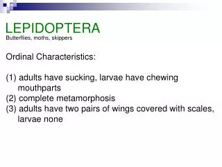
Lepidoptera • Lepidoptera is second largest class in Insecta • Approximately 600 species of moths occur in the H.J. Andrews Experimental Forest • Relatively little is known
Ecosystem Functions Prey Diverse Ecological Roles Defoliators Pollinators Decomposers Stages of lifecycle Moth Egg Caterpillar Pupa
Prey Pollination Ecosystem connections Rodents Reptiles 570 vascular plant species True bugs Bats Spiders Nematodes Birds Beetles
Assessing Environmental Impacts Source of food, impacted by abundance of food source, sensitive to changes in temperature and nutritional quality of plants . Temperature Plant Nutrition Sensitive to nitrogen and water content High water content enhances growth Theoretically, moth abundance and/or emergence could be linked to changes in nitrogen and water content of plants. • Caterpillar growth rate affected by temperature • Caterpillar must reach certain critical size to enter pupal stage • Majority of moths in Pacific northwest overwinter as egg or in cocoon • Many species won’t emerge unless undergo period of cold (dipause)
Moth Sampling • Universal Black light traps • 22w circular bulbs, 12v batteries • Set 1 – 2 hours before sunset • Moths attracted to light and stunned by insecticide and acrylic veins • Intervals of 1+ weeks • Biased towards phototatic night flying moths (majority) • Data not used this summer, will be used in island biogeography study
Moth Data Used in Modeling • Sampled with same method by Jeffrey Miller 2004-2008 • Emergence uses data from 20 sites trapped 30+ times • Moth Distribution includes data from biological inventory survey • Almost 40% sites trapped only once • More than half trapped either once or twice Feraliadeceptiva
Vegetation Sampling • Purpose: Test hypothesis that moths are distributed near host plants by contributing to a database of vegetation data at moth sampling sites • 32 sites • 100 meters in 4 directions • All vascular plant species except fern allies (except horsetails) • To learn more about host plants Polystichummunitum
Phenology and Climate Change • “As difficult as it is to predict precisely how the planet will warm over the next century or so, it is even harder to refine predictions of how those changes will affect specific species.”1 • What are the drivers of moth emergence? • Moths are poikilothermic • How will climate change influence moth emergence? • “Due to human induced climate change over the last decade, phenology has become one of the leading indicators of species’ response to environmental change”2 • Will this have an effect on other animals? 1: Barringer, Felicity. “Trout Fishing in a Climate Changed America.” New York Times Green Blog16/7/2011. 16/7/2011. 2: Roy, DB & Sparks, TH. “Phenologyof British butterflies and climate change.” Global Change Biology (2000). 6, 407-416.
Emergence Objectives • Improve on the previous model • Create a model that can predict on which day moths will emerge • Use degree days instead of Julian days: GDD for plants
Model Counts with Julian Days as the interval Degree-Day Curve Model Model Showing Counts with Degree Days as interval
Degree Days • Took max temp. data from HJ Andrews • Assigned trap sites to Met. and Ref. Stands • Interpolated missing data • Discuss procedure for calculations
Thermal Climate of the H.J. Andrews Experimental Forest PRISM estimated mean monthly maximum and minimum temperature maps showing topographic effects of radiation and sky view factors. Provided by Jonathan W. Smith and EISI 2010
Formula:=IF(‘VANMET’!B4>0,’VANMET’!B4,0)+'VANMET DEGREE DAYS'!B2
The Model • Uses abundance data from trapping • Estimates parameters of emergence and abundance curves from trap counts • Optimizes parameter estimates to create emergence and abundance curves
P(j,k) • We assume we catch all moths flying at trap time • P(j,k) is the probability that a moth emerges in interval j and has a natural death time in interval k • Measures abundance
Variables Emergence time: Lifespan: • In original model, P(j,k) found by numerically integrating the joint density • Q(j,k) and qj successively computed • Likelihood function uses qj to optimize parameter estimates
Obtaining our parameters = Pr(moth caught by trap) m = # moths flying qj = Pr(moth trapped at tj) Assume (a constant)
Convergence in distribution As and , we assume (expected value of moths caught) approaches some constant . . . Where the Fi’s are Poisson random variables
Distribution, cont. • m and alpha are unknown • If m is large and alpha small enough, the likelihood will be very close to Poisson • The model uses the multinomial distribution :
Incorporating degree days • Degree day values: • Each moth has emergence threshold, D • Now define
Changes • Compute P(j,k) differently because Te is discrete • Single set of parameters for each species, rather than separate for each trap and year • AIC: measure of fit
3G Days Since May 1st 3G Degree Days
5O Days Since May 1st 5O Degree Days
Future Work • Degree Days • Revisit interpolation methods • Experiment with different degree thresholds and starting dates • Model • Multinomial v. Poisson • Multiple traps for one year • Take new data into account: • Vegetation surveys • Elevation, Aspect, Watershed, Habitat
Species Distribution Model Applications • Combine numerical observations and relevant variables (often environmental and spatial) to predict species distribution in space and/or time • Why do this? • Ecological insight, further research topics • Land use management and conservation planning
SDM’s and Machine Learning • Supervised machine learning • Use training data: {(x1,y1), (x2,y2),…,(xn,yn)} to arrive at a function f(xi) ≈ yi. • Split data into training, test, and validation sets. • Assume that if a moth exists at each site we’ve trapped it at least once at that site.
SDM’s and Machine Learning • Training set: half of the original data set used in initially learning and fitting the function. • Certain algorithms require their parameters to be tuned for optimum performance. This is accomplished by testing the model against a validation set – a subset of the training set. • Test set: half of the original data set separate from the training set. • After parameter tuning, the function’s accuracy can be evaluated by running it on a test set.
Quantifying Accuracy • The area under the receiver operating characteristic curve (AUC) is used as our measure of accuracy for the distribution maps. • It is the probability that a randomly selected positive instance (moth presence) is ranked higher than a randomly selected negative instance. • AUC = 0.5 indicates a random guess.
Learning Algorithms Algorithms Corresponding R package randomForest glmnet e1071 gbm • Random Forest • Logistic Regression • Support Vector Machines • Generalized Boosted Regression Models
Random Forest • Ensemble method • Grows decision trees by combining “bagging” with the random selection of features. • A decision tree is a model of decisions and their outcomes. Internal nodes represent points where a decision is made, and the leaves represent the outcomes. • “Bagging” is the process of randomly sampling with replacement from the set of training examples, and constructing a decision tree from the “bag”. • Random forest also randomly selects features for each training example rather using the whole of features.
Random Forest Plant #1 False True Plant #2 Pred #1 False True False True Absent Present Present Temp Low High Absent Present
Tuning Random Forest • After creating n bags, and growing n trees new data can be classified by taking a vote of all the trees’ predictions. • The number of trees grown can be altered and tuned as can the number of nodes of each tree.
Logistic Regression • P(y = 1|x) = 1/(1+e-t) • Where tis (β0 + β1x1 +…+ βnxn) • Attempt to find appropriate β values to weigh the covariates.
Tuning Logistic Regression • It is oftentimes optimal to restrict the number and size of these β values in regression. There is a combination of penalty terms called the “elastic net” to achieve these restrictions. • Penalty term takes the form: λ[((1-α)/2)*|β|2 + (α*|β|)] • The parameters: α and λ are tuned. • α controls which term is more important. • λ controls the weight of the entire expression.
Support Vector Machines • Non-probabilistic classifier. • Attempts to construct an n-dimensional hyperplaneto separate two possible classes of data. • The most desirable hyperplane is the one with the largest functional margin.
Tuning Support Vector Machines • Oftentimes data is not linearly separable. • Kernel functions map the data unto a space where a hyperplane can be easily constructed. • Linear • Radial • Sigmoid • Polynomial
Generalized Boosted Regression Models • Ensemble Method • Loss function: a measure that represents the loss in predictive performance of a model. • GBM’s construct an initial regression tree that maximally reduces the loss function. • A regression tree is a decision tree whose outputs are real-valued.
Generalized Boosted Regression Models • To further reduce the loss function, new trees are added. • At the second step, a regression tree is fitted using the residuals (variations in response) of the first tree. • The model now updates to contain two terms, and residuals are taken from the two-term model. The process continues in this stage-wise fashion until a specified parameter – n.trees. • Fitted values update with each new tree addition.
Tuning GBM • Like the other learning algorithms, GBM also has parameters to be tuned. • The number of trees to be constructed and added. • The number of nodes in each tree (interaction depth).
Algorithm Performance Logistic Regression Random Forest Avg AUC = .607 Avg AUC = .605 gbm SVM Avg AUC = .505 Avg AUC = .606
Acknowledgements • NSF • OSU • OSU Arthropod Museum • Matt Cox • Steve Highland • Tom Dietterich • Dan Sheldon • Olivia Poblacion • Julia Jones • Desiree Tullos • Jorge Ramirez • John & Emily • Vera • Jeff Miller/Paul C. Hammond