Download
1 / 100
1k likes | 1.15k Views
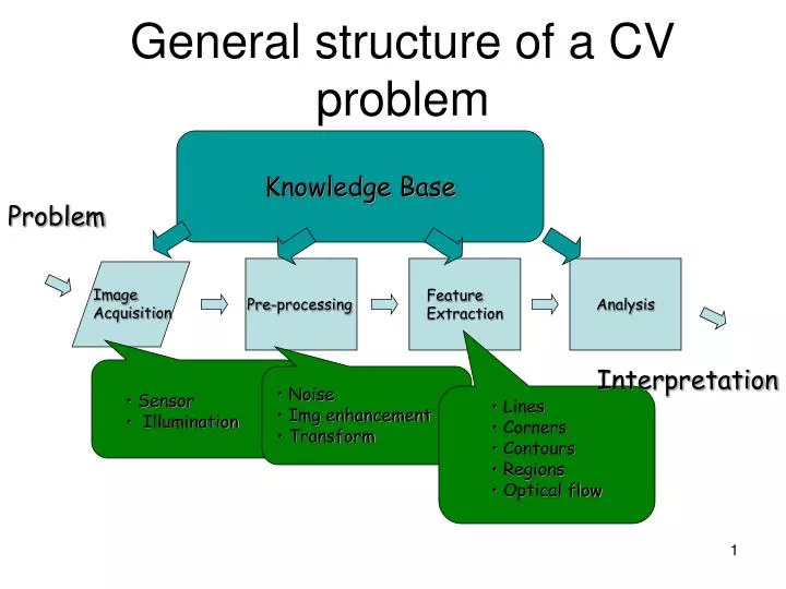
Analysis. Pre-processing. Image Acquisition. Noise Img enhancement Transform. Sensor Illumination. Lines Corners Contours Regions Optical flow. Feature Extraction. Knowledge Base. General structure of a CV problem. Problem. Interpretation. Digital Images.

E N D
Analysis Pre-processing Image Acquisition • Noise • Img enhancement • Transform • Sensor • Illumination • Lines • Corners • Contours • Regions • Optical flow Feature Extraction Knowledge Base General structure of a CV problem Problem Interpretation
Digital Images are 2D arrays (matrices) of numbers:
Why do we need Linear Algebra? • We will associate coordinates to • 3D points in the scene • 2D points in the CCD array • 2D points in the image • Coordinates will be used to • Perform geometrical transformations • Associate 3D with 2D points • Images are matrices of numbers • We will find properties of these numbers
2D Translation P’ t P
P’ t ty P y x tx 2D Translation using Homogeneous Coordinates t P
Scaling P’ P
Scaling Equation P’ Sy.y P y x Sx.x
S T Scaling & Translating P’’=T.P’ P’=S.P P P’’=T.P’=T.(S.P)=(T.S).P
Scaling & Translating P’’=T.P’=T.(S.P)=(T.S).P
Rotation P P’
P’ Y’ g P y x X’ 3D Rotation of Points Rotation around the coordinate axes, counter-clockwise: z
Scaling, Translating & Rotating Order matters! P’ = S.P P’’=T.P’=(T.S).P P’’’=R.P”=R.(T.S).P=(R.T.S).P R.T.S R.S.T T.S.R …
4-neighbors 8-neighbors Digital Images • Array of numbers (pixels) • Typically integers 0-255 (unsigned byte) • Pixels have neighbors
4-connected path 8-connected path Image Paths • A path is a sequence of pixel indices (io,jo)(i1,j1)…(in,jn) such that (ik,jk) is a neighbor of (ik+1,jk+1)
Levels of Computation • Point level • Output based only on a single point • Ex.: thresholding • Local level • Output based on a neighborhood • Ex. : smoothing and edge detection • Global level • Output based on the whole image • Ex.: Fourier transform and histogram • Object level • Output based on pixels that belong to an object
Image Noise • Images are noisy • Noise is anything in the image that we are not interested in • Examples: • Fluctuations of pixel values • Numerical errors
Where does noise come from? • Light fluctuations • Sensor noise • Quantization effects • Finite precision
Filter F I= Î+N O F a c b d f g h i Linear Filtering O, NxM output image I, NxM input image F mxm mask: (m odd) e
11 10 0 0 1 10 X X X X X X 10 1 0 1 9 11 10 X X 10 10 9 0 2 1 I X X 11 10 9 9 11 10 X X 9 10 11 9 99 11 X X 10 9 9 11 10 10 X X X X X X Example: O F 1 1 1 1 1 1 1/9 1 1 1 1/9.(10x1 + 11x1 + 10x1 + 9x1 + 10x1 + 11x1 + 10x1 + 9x1 + 10x1) = 1/9.( 90) = 10
Example: X X X X X X 11 10 0 0 1 10 7 4 1 10 X X 10 1 0 1 9 11 O X X 10 10 9 0 2 1 I X X 11 10 9 9 11 10 F X X 9 10 11 9 99 11 X X X X X X 10 9 9 11 10 10 1 1 1 1 1 1 1/9 1 1 1 1/9.(10x1 + 0x1 + 0x1 + 11x1 + 1x1 + 0x1 + 10x1 + 0x1 + 2x1) = 1/9.( 34) = 3.7778
F 1 1 1 1 1 1 1 1 1 Example: X X X X X X 11 10 0 0 1 10 7 4 1 10 X X 10 1 0 1 9 11 O X X 10 10 9 0 2 1 I X X 11 10 9 9 11 10 X 20 X 9 10 11 9 99 11 X X X X X X 10 9 9 11 10 10 1/9 1/9.(10x1 + 9x1 + 11x1 + 9x1 + 99x1 + 11x1 + 11x1 + 10x1 + 10x1) = 1/9.( 180) = 20
F 1 1 1 1 1 1 1 1 1 Example: X X X X X X 11 10 0 0 1 10 7 4 1 10 X X 10 1 0 1 9 11 O X X 10 10 9 0 2 1 I X 18 X 11 10 9 9 11 10 X 20 X 9 10 11 9 99 11 X X X X X X 10 9 9 11 10 10 1/9 1/9.(10x1 + 0x1 + 2x1 + 9x1 + 10x1 + 9x1 + 11x1 + 9x1 + 99x1) = 1/9.( 159) = 17.6667
How big should the mask be? • The bigger the mask, • more neighbors contribute. • smaller noise variance of the output. • bigger noise spread. • more blurring. • more expensive to compute.
Gaussian Filter • A particular case of averaging • The coefficients are a 2D Gaussian. • Gives more weight at the central pixel and less weights to the neighbors. • The farther away the neighbors, the smaller the weight.
Non-linear Filtering • Replace each pixel with the MEDIAN value of all the pixels in the neighborhood.
11 10 0 0 1 10 X X X X X X 10 1 0 1 9 11 10 X X 10 10 9 0 2 1 I X X 11 10 9 9 11 10 X X 9 10 11 9 99 11 X X 10 9 9 11 10 10 X X X X X X Example: O median sort 10,11,10,9,10,11,10,9,10 9,9,10,10,10,10,10,11,11
Example: 11 10 0 0 1 X X X X X 10 X 1 1 10 1 0 1 10 X 9 11 10 X O 10 10 9 0 2 1 X X I 11 10 9 9 11 X X 10 9 10 11 9 99 11 X X 10 9 9 11 10 10 X X X X X X median sort 11,10,0,10,11,1,9,10,0 0,0,1,9,10,10,10,11,11
Example: X X X X X X 11 10 0 0 1 10 10 X X 10 1 0 1 9 11 O X X 10 10 9 0 2 1 I 9 X X 11 10 9 9 11 10 X X 10 9 10 11 9 99 11 X X X X X X 10 9 9 11 10 10 median sort 10,9,11,9,99,11,11,10,10 9,9,10,10,10,11,11,11,99
Median Filter Properties • Non-linear • Does not spread the noise • Can remove spike noise • Expensive to run
Regions and Edges • Ideally, regions are bounded by closed contours • We could “fill” closed contours to obtain regions • We could “trace” regions to obtain edges • Unfortunately, these procedures rarely produce satisfactory results.
Regions and Edges • Edges are found based on DIFFERENCES between values of adjacent pixels. • Regions are found based on SIMILARITIES between values of adjacent pixels.
Number of pixels Gray value T Histogram-based Segmentation • Select threshold • Create binary image: • I(x,y) < T -> O(x,y) = 0 • I(x,y) > T -> O(x,y) = 1 Ex: bright object on dark background: Histogram
Algorithm MEAN SHIFT for Image Segmentation • Find image histogram, choose window size • Choose initial location of search window: • Randomly select a number M of image pixels • Find the average value in a 3x3 window for each of these pixels • Set the center of the window to the value with largest histogram count. • Apply mean shift to find the window peak. • Remove pixels in the window from the image and the histogram. • Repeat steps 2 to 4 until no pixels are left.
Iterative Threshold Algorithm • Select initial T = To • Ex: To = average intensity • Partition image into regions R1 and R2 using T • Calculate the mean values of R1 and R2, m1 and m2 • Select a new threshold T = ½(m1 + m2) • Repeat 2-4 until m1 and m2 do not change.
Limitations of histogram methods: • Use GLOBAL information • Ignore SPATIAL relationships among pixels.
SPLIT & MERGE Algorithms • Simple intensity algorithms usually result in too many regions. • Reasons: • high frequency noise • Gradual transitions between regions • After segmentation, regions might need refinement: • Interactively or automatically • May use domain and or image process knowledge
1 2 3 4 Merging Algorithm • Start with an initial segmentation • Ex: • By thresholding, • nxn (5x5, 7x7, etc) regions • manually selected • Each region has a unique “label”
1 2 3 4 Merging Algorithm • Form the Region Adjacency Graph • Regions are the nodes • Adjacency relations are the links
1 2 4 Merging Algorithm • For each region in the image do: • Consider its adjacent regions and test if they are similar • If they are similar, merge them and update the RAG
1 2 4 Merging Algorithm • Repeat the previous step until there are no more merges.
Split and Merge Algorithms • Split and merge are often used together: • Start with the initial image and a “predicate” • Test the image with the predicate: • If it doesn’t satisfy it, split image into quarters; • Repeat for each sub-region until there are no more splits. • Test adjacent regions with the predicate: • If they satisfy it: merge them.
1 1 1 1 1 2 2 2 2 2 3 3 3 3 3 4 4 4 4 4 Split …
1 1 1 2 2 2 3 3 3 4 4 4 Merge …
Quadtree Representation • Quadtrees: • Trees where nodes have 4 children • Build quadtree: • Nodes represent regions • Every time a region is split, it’s node gives birth to 4 children • Leaves are nodes for uniform regions • Merging: • Siblings that are “similar” can be merged.
Gray value column column Edge Edge Edges • They happen at places where the image values exhibit sharp variation
Edge detection (1D) F(x) Edge= sharp variation x F ’(x) Large first derivative x
y F(x) x x dI(x) dI(x) dx dx > Th Edge Detection (2D) 1D 2D I(x) I(x,y) I(x,y)=[I(x,y)/x I(x,y)/y]t = [Ix(x,y) Iy(x,y)]t |I(x,y)| =(Ix 2(x,y) + Iy2(x,y))1/2 > Th tan = Ix(x,y)/ Iy(x,y)
Noise Filter Edge Detection Noise cleaning and Edge Detection E(x,y) I(x,y) Combine Linear Filters
-1 -1 -1 0 0 0 1 1 1 Noise Smoothing & Edge Detection Convolve with: Noise Smoothing Vertical Edge Detection This mask is called the (vertical) Prewitt Edge Detector
-1 0 1 -1 0 1 -1 0 1 Noise Smoothing & Edge Detection Convolve with: Horizontal Edge Detection Noise Smoothing This mask is called the (horizontal) Prewitt Edge Detector