Download

1 / 61
610 likes | 632 Views
Discover the different types of forecasting models - time series, causal, and qualitative. Learn about methods like Delphi, consumer surveys, and executive opinions. Evaluate forecast accuracy with measures like MAD, MSE, and MAPE.

E N D
Chapter 5 Forecasting
Eight Steps to Forecasting 1. Determine the use of the forecast—what objective are we trying to obtain? 2. Select the items or quantities that are to be forecasted. 3. Determine the time horizon of the forecast—is it 1 to 30 days (short term), 1 month to 1 year (medium term), or more than 1 year (long term)? 4. Select the forecasting model or models. 5. Gather the data or information needed to make the forecast. 6. Validate the forecasting model. 7. Make the forecast. 8. Implement the results. 5-2
Time-Series Models • Time-series models attempt to predict the future by using historical data. • In other words, time-series models look at what has happened over a period of time and use a series of past data to make a forecast. • The time-series models we examine in this chapter are • Moving average • Exponential smoothing, • Trend projections, and • Decomposition. Regression analysis can be used in trend projections and is one type of decomposition model. The primary emphasis of this chapter is time series forecasting. 5-4
Causal Models • Causal models incorporate the variables or factors that might influence the quantity being forecasted into the forecasting model. For example, daily sales of a cola drink might depend on the season, the average temperature, the average humidity, whether it is a weekend or a weekday, and so on. • Causal models may also include past sales data as time-series models do, but they include other factors as well. • These include • Linear regression analysis • Multiple regression analysis 5-5
Qualitative Models • Qualitative models attempt to incorporate judgmental or subjective factors into the forecasting model. • Opinions by experts, individual experiences and judgments, and other subjective factors may be considered. • Qualitative models are especially useful when subjective factors are expected to be very important or when accurate quantitative data are difficult to obtain. 5-6
Delphi method. • This iterative group process allows experts, who may be located in different places, to make forecasts. • There are three different types of participants in the Delphi process: decision makers, staff personnel, and respondents. • The decision making group usually consists of 5 to 10 experts who will be making the actual forecast. • The staff personnel assist the decision makers by preparing, distributing, collecting, and summarizing a series of questionnaires and survey results. • The respondents are a group of people whose judgments are valued and are being sought. This group provides inputs to the decision makers before the forecast is made. 5-7
Jury of executive opinion • This method takes the opinions of a small group of high-level managers, often in combination with statistical models, and results in a group estimate of demand. 5-8
Sales force composite • In this approach, each salesperson estimates what sales will be in his or her region; these forecasts are reviewed to ensure that they are realistic and are then combined at the district and national levels to reach an overall forecast. 5-9
Consumer market survey • This method solicits input from customers or potential customers regarding their future purchasing plans. • It can help not only in preparing a forecast but also in improving product design and planning for new products. 5-10
Scatter Diagrams and Time Series • A scatter diagram helps to obtain ideas about a relationship. 5-11
Measures of Forecast Accuracy Forecast error = Actual value - Forecast value Mean Absolute Deviation (MAD). This is computed by taking the sum of the absolute values of the individual forecast errors and dividing by the numbers of errors (n): 5-15
Mean Squared Error (MSE), • It is the average of the squared errors 5-17
Mean Absolute Percent Error (MAPE) • The MAPE is the average of the absolute values of the errors expressed as percentages of the actual values. 5-18
Components of a Time Series • 1. Trend (T) is the gradual upward or downward movement of the data over time. • 2. Seasonality (S) is a pattern of the demand fluctuation above or below the trend line that repeats at regular intervals. • 3. Cycles (C) are patterns in annual data that occur every several years. They are usually tied into the business cycle. • 4. Random variations (R) are “blips” in the data caused by chance and unusual situations; they follow no discernible pattern. 5-19
Moving Averages 5-21
Exponential Smoothing • Exponential smoothing is a type of moving average technique, which involves little record keeping of past data. The exponential smoothing approach has been applied successfully by banks, manufacturing companies, wholesalers, and other organizations. The exponential smoothing formula is as follow: 5-26
Example • In January, a demand for 142 of a certain car model for February was predicted by a dealer. Actual February demand was 153 autos. Using a smoothing constant of we can forecast the March demand using the exponential smoothing model. 5-28
SELECTING THE SMOOTHING CONSTANT • The appropriate value of the smoothing constant can make the difference between an accurate forecast and an inaccurate forecast. • In picking a value for the smoothing constant, the objective is to obtain the most accurate forecast. • Several values of the smoothing constant may be tried, and the one with the lowest MAD could be selected. • This is analogous to how weights are selected for a weighted moving average forecast. • Some forecasting software automatically select the best smoothing constant. • QM for Windows displays the MAD that obtains values of ranging from 0 to 1 in increments of 0.01. 5-29
Example 5-30
EXPONENTIAL SMOOTHING WITH TREND ADJUSTMENT • The averaging or smoothing forecasting techniques are useful when a time series has random component, but these techniques are not suitable to respond trends. • The idea is to develop an exponential smoothing forecast and then adjust this for trend. • Two smoothing constants, and are used in this model, and both of these values must be between 0 and 1. The level of the forecast is adjusted by multiplying the first smoothing constant, by the most recent forecast error and adding it to the previous forecast. • The trend is adjusted by multiplying the second smoothing constant, by the most recent error or excess amount in the trend. • A higher value gives more weight to recent observations and thus responds more quickly to changes in the patterns. 5-32
Trend Projection Trend projections are used to forecast time-series data that exhibit a linear trend. • Least squares may be used to determine a trend projection for future forecasts. • Least squares determines the trend line forecast by minimizing the mean squared error between the trend line forecasts and the actual observed values. • The independent variable is the time period and the dependent variable is the actual observed value in the time series. 5-38
Trend Projection (continued) The formula for the trend projection is: Y= b + b X where: Y = predicted value b1 = slope of the trend line b0 = intercept X = time period (1,2,3…n) 0 1 5-39
Midwestern Manufacturing Trend Projection Example Midwestern Manufacturing Company’s demand for electrical generators over the period of 2004 – 2010 is given below. 5-40
Midwestern Manufacturing Company Trend Solution Sales = 56.71 + 10.54 (time) 5-42
Seasonal Variations Seasonal indices can be used to make adjustments in the forecast for seasonality. • A seasonal index indicates how a particular season compares with an average season. • The seasonal index can be found by dividing the average value for a particular season by the average of all the data. 5-44
Now suppose we expected the third year’s annual demand for answering machines to be 1,200 units, which is 100 per month. We would not forecast each month to have a demand of 100, but we would adjust these based on the seasonal indices as follows: 5-46
Average Average Month Sales Demand Seasonal Two-Year Monthly Index Demand Demand Year 1 Year 2 Jan 90 94 0.957 80 100 Feb 75 85 80 94 0.851 Mar 80 90 85 94 0.904 Apr 90 110 100 94 1.064 May 115 131 123 94 1.309 … … … … … … Total Average Demand 1,128 Seasonal Index: = Average 2 -year demand/Average monthly demand Eichler Supplies: Seasonal Index Example 5-48
Seasonal Variations with Trend Centered Moving Average (CMA) is an approach that prevents a variation due to trend from being incorrectly interpreted as a variation due to the season. Steps of Multiplicative Time-Series Model1. Compute the CMA for each observation. • Compute seasonal ratio (observation/CMA). 3. Average seasonal ratios to get seasonal indices. 4. If seasonal indices do not add to the number of seasons, multiply each index by (number of seasons)/(sum of the indices). 5-49