Download
1 / 49
490 likes | 635 Views
02/14/12. Fitting and Registration. Computer Vision CS 543 / ECE 549 University of Illinois Derek Hoiem. Announcements. HW 1 due today Early feedback form. Fitting: find the parameters of a model that best fit the data

E N D
02/14/12 Fitting and Registration Computer Vision CS 543 / ECE 549 University of Illinois Derek Hoiem
Announcements • HW 1 due today • Early feedback form
Fitting: find the parameters of a model that best fit the data Alignment: find the parameters of the transformation that best align matched points
Fitting and Alignment • Design challenges • Design a suitable goodness of fit measure • Similarity should reflect application goals • Encode robustness to outliers and noise • Design an optimization method • Avoid local optima • Find best parameters quickly
Fitting and Alignment: Methods • Global optimization / Search for parameters • Least squares fit • Robust least squares • Iterative closest point (ICP) • Hypothesize and test • Generalized Hough transform • RANSAC
Least squares line fitting • Data: (x1, y1), …, (xn, yn) • Line equation: yi = mxi + b • Find (m, b) to minimize y=mx+b (xi, yi) Matlab: p = A \ y; Modified from S. Lazebnik
Problem with “vertical” least squares • Not rotation-invariant • Fails completely for vertical lines Slide from S. Lazebnik
Slide modified from S. Lazebnik Total least squares If (a2+b2=1) then Distance between point (xi, yi) is |axi + byi + c| ax+by+c=0 Unit normal: N=(a, b) (xi, yi) proof: http://mathworld.wolfram.com/Point-LineDistance2-Dimensional.html
Slide modified from S. Lazebnik Total least squares If (a2+b2=1) then Distance between point (xi, yi) is |axi + byi + c| Find (a, b, c) to minimize the sum of squared perpendicular distances ax+by+c=0 Unit normal: N=(a, b) (xi, yi)
Slide modified from S. Lazebnik Total least squares Find (a, b, c) to minimize the sum of squared perpendicular distances ax+by+c=0 Unit normal: N=(a, b) (xi, yi) Solution is eigenvector corresponding to smallest eigenvalue of ATA See details on Raleigh Quotient: http://en.wikipedia.org/wiki/Rayleigh_quotient
Recap: Two Common Optimization Problems Problem statement Solution Problem statement Solution (matlab)
Least squares (global) optimization Good • Clearly specified objective • Optimization is easy Bad • May not be what you want to optimize • Sensitive to outliers • Bad matches, extra points • Doesn’t allow you to get multiple good fits • Detecting multiple objects, lines, etc.
Robust least squares (to deal with outliers) General approach: minimize ui(xi, θ) – residual of ith point w.r.t. model parameters θρ – robust function with scale parameter σ • The robust function ρ • Favors a configuration • with small residuals • Constant penalty for large residuals Slide from S. Savarese
Robust Estimator • Initialize: e.g., choose by least squares fit and • Choose params to minimize: • E.g., numerical optimization • Compute new • Repeat (2) and (3) until convergence
Other ways to search for parameters (for when no closed form solution exists) • Line search • For each parameter, step through values and choose value that gives best fit • Repeat (1) until no parameter changes • Grid search • Propose several sets of parameters, evenly sampled in the joint set • Choose best (or top few) and sample joint parameters around the current best; repeat • Gradient descent • Provide initial position (e.g., random) • Locally search for better parameters by following gradient
Hypothesize and test • Propose parameters • Try all possible • Each point votes for all consistent parameters • Repeatedly sample enough points to solve for parameters • Score the given parameters • Number of consistent points, possibly weighted by distance • Choose from among the set of parameters • Global or local maximum of scores • Possibly refine parameters using inliers
Hough Transform: Outline • Create a grid of parameter values • Each point votes for a set of parameters, incrementing those values in grid • Find maximum or local maxima in grid
Hough transform P.V.C. Hough, Machine Analysis of Bubble Chamber Pictures, Proc. Int. Conf. High Energy Accelerators and Instrumentation, 1959 Given a set of points, find the curve or line that explains the data points best y m b x Hough space y = m x + b Slide from S. Savarese
y m 3 5 3 3 2 2 3 7 11 10 4 3 2 3 1 4 5 2 2 1 0 1 3 3 x b Hough transform y m b x Slide from S. Savarese
Hough transform P.V.C. Hough, Machine Analysis of Bubble Chamber Pictures, Proc. Int. Conf. High Energy Accelerators and Instrumentation, 1959 Issue : parameter space [m,b] is unbounded… Use a polar representation for the parameter space y x Hough space Slide from S. Savarese
Hough transform - experiments votes features Slide from S. Savarese
Hough transform - experiments Noisy data Need to adjust grid size or smooth features votes Slide from S. Savarese
Hough transform - experiments Issue: spurious peaks due to uniform noise features votes Slide from S. Savarese
3. Hough votes Edges Find peaks and post-process
Hough transform example http://ostatic.com/files/images/ss_hough.jpg
Finding lines using Hough transform • Using m,b parameterization • Using r, theta parameterization • Using oriented gradients • Practical considerations • Bin size • Smoothing • Finding multiple lines • Finding line segments
Finding circles (x0, y0, r) using Hough transform • Fixed r • Variable r
Hough transform conclusions Good • Robust to outliers: each point votes separately • Fairly efficient (much faster than trying all sets of parameters) • Provides multiple good fits Bad • Some sensitivity to noise • Bin size trades off between noise tolerance, precision, and speed/memory • Can be hard to find sweet spot • Not suitable for more than a few parameters • grid size grows exponentially Common applications • Line fitting (also circles, ellipses, etc.) • Object instance recognition (parameters are affine transform) • Object category recognition (parameters are position/scale)
RANSAC (RANdom SAmple Consensus) : Fischler & Bolles in ‘81. • Algorithm: • Sample (randomly) the number of points required to fit the model • Solve for model parameters using samples • Score by the fraction of inliers within a preset threshold of the model • Repeat 1-3 until the best model is found with high confidence
RANSAC Line fitting example • Algorithm: • Sample (randomly) the number of points required to fit the model (#=2) • Solve for model parameters using samples • Score by the fraction of inliers within a preset threshold of the model • Repeat 1-3 until the best model is found with high confidence Illustration by Savarese
RANSAC Line fitting example • Algorithm: • Sample (randomly) the number of points required to fit the model (#=2) • Solve for model parameters using samples • Score by the fraction of inliers within a preset threshold of the model • Repeat 1-3 until the best model is found with high confidence
RANSAC Line fitting example • Algorithm: • Sample (randomly) the number of points required to fit the model (#=2) • Solve for model parameters using samples • Score by the fraction of inliers within a preset threshold of the model • Repeat 1-3 until the best model is found with high confidence
RANSAC • Algorithm: • Sample (randomly) the number of points required to fit the model (#=2) • Solve for model parameters using samples • Score by the fraction of inliers within a preset threshold of the model • Repeat 1-3 until the best model is found with high confidence
How to choose parameters? • Number of samples N • Choose N so that, with probability p, at least one random sample is free from outliers (e.g. p=0.99) (outlier ratio: e ) • Number of sampled points s • Minimum number needed to fit the model • Distance threshold • Choose so that a good point with noise is likely (e.g., prob=0.95) within threshold • Zero-mean Gaussian noise with std. dev. σ: t2=3.84σ2 modified from M. Pollefeys
RANSAC conclusions Good • Robust to outliers • Applicable for larger number of objective function parameters than Hough transform • Optimization parameters are easier to choose than Hough transform Bad • Computational time grows quickly with fraction of outliers and number of parameters • Not good for getting multiple fits Common applications • Computing a homography (e.g., image stitching) • Estimating fundamental matrix (relating two views)
What if you want to align but have no prior matched pairs? • Hough transform and RANSAC not applicable • Important applications Medical imaging: match brain scans or contours Robotics: match point clouds
Iterative Closest Points (ICP) Algorithm Goal: estimate transform between two dense sets of points • Initialize transformation (e.g., compute difference in means and scale) • Assigneach point in {Set 1} to its nearest neighbor in {Set 2} • Estimate transformation parameters • e.g., least squares or robust least squares • Transform the points in {Set 1} using estimated parameters • Repeat steps 2-4 until change is very small
Algorithm Summary • Least Squares Fit • closed form solution • robust to noise • not robust to outliers • Robust Least Squares • improves robustness to noise • requires iterative optimization • Hough transform • robust to noise and outliers • can fit multiple models • only works for a few parameters (1-4 typically) • RANSAC • robust to noise and outliers • works with a moderate number of parameters (e.g, 1-8) • Iterative Closest Point (ICP) • For local alignment only: does not require initial correspondences
Example: solving for translation A1 B1 A2 B2 A3 B3 Given matched points in {A} and {B}, estimate the translation of the object
Example: solving for translation (tx, ty) A1 B1 A2 B2 A3 B3 Least squares solution • Write down objective function • Derived solution • Compute derivative • Compute solution • Computational solution • Write in form Ax=b • Solve using pseudo-inverse or eigenvalue decomposition
Example: solving for translation A5 B4 (tx, ty) A1 B1 A4 B5 A2 B2 A3 B3 Problem: outliers RANSAC solution Sample a set of matching points (1 pair) Solve for transformation parameters Score parameters with number of inliers Repeat steps 1-3 N times
Example: solving for translation (tx, ty) A4 B4 B1 A1 A2 B2 B5 A5 A3 B3 B6 A6 Problem: outliers, multiple objects, and/or many-to-one matches Hough transform solution Initialize a grid of parameter values Each matched pair casts a vote for consistent values Find the parameters with the most votes Solve using least squares with inliers
Example: solving for translation (tx, ty) Problem: no initial guesses for correspondence ICP solution Find nearest neighbors for each point Compute transform using matches Move points using transform Repeat steps 1-3 until convergence
Next class: Object Recognition • Keypoint-based object instance recognition and search