Download
1 / 35
350 likes | 463 Views
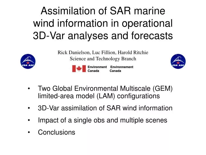
Rick Danielson, Luc Fillion, Harold Ritchie Science and Technology Branch. Assimilation of SAR marine wind information in operational 3D-Var analyses and forecasts. Two Global Environmental Multiscale (GEM) limited-area model (LAM) configurations 3D-Var assimilation of SAR wind information

E N D
Rick Danielson, Luc Fillion, Harold Ritchie Science and Technology Branch Assimilation of SAR marinewind information in operational3D-Var analyses and forecasts • Two Global Environmental Multiscale (GEM) limited-area model (LAM) configurations • 3D-Var assimilation of SAR wind information • Impact of a single obs and multiple scenes • Conclusions
Clipped observations assimilated on Feb 10, 2009 (9-15 UTC)
Operational GEM-LAM Configuration • Forecast • Uniform 649 x 672 grid at • 15-km resolution, 80 levels • Analysis • 3D-Var at 55-km • resolution • Hemispheric spherical- • harmonic representation • Dynamical balance • enforced directly from • spectral cross-correlations Fillion et al. (Wea. Forecasting 2010)
2.5-km windows (summer 2010) Experimental GEM-LAM Configuration • Forecast • Uniform grids at 2.5-km • resolution, 58 levels • Proposed Analysis • 3D-Var at 15-km resolution • Non-separable background • error correlations using a • bi-Fourier representation • Dynamical balance • enforced directly from • spectral cross-correlations
Experimental GEM-LAM Configuration Operational Analysis (55-km) Forecast (15-km) Proposed Analysis and Pilot Forecast (15-km) Experimental Forecast (2.5-km)
Experimental GEM-LAM Configuration GEM Pilot UTC • 10 Nov – 20 Dec 2009 • 209 Radarsat-2 scenes (10/22 UTC) • 60 assimilation periods (12/00 UTC) • 46 buoy platforms (not assimilated) 3DVar 15km 06 09 12 15 18 21 00 03 06 09 12 GEM 2.5km (FGAT) 1h @ 144 CPUs 20min @ 64 CPUs
Find best fit to observations and model, taking into account their statistical errors 3D-Var assimilation of SAR • Least squares approach: X = Pilot Forecast y = (SAR) Obs Δx = Correction to X 2 2 Misfit between X + Δx and X Misfit between X + Δx and y J(Δx) = + Statistical errors of X Statistical errors of y
Find best fit to observations and model, taking into account their statistical errors 3D-Var assimilation of SAR • Least squares approach: • Analysis (X+Δx) outcomes: X = Pilot Forecast y = (SAR) Obs Δx = Correction to X 2 2 Misfit between X + Δx and X Misfit between X + Δx and y J(Δx) = + Statistical errors of X Statistical errors of y LARGE X errors and smally errors : Analysis≈ y smallX errors and LARGE y errors : Analysis ≈ X
3D-Var assimilation of SAR • SAR misfit calculation: • a) interpolate analysis winds (X+Δx) from • ~40m (lowest active model level) to 10m • b) apply a C-band model function (CMOD5; • Hersbach et al. 2007) for VV polarization • and include a polarization ratio (Mouche • et al. 2005) for HH • c) compare to Radarsat-2 SAR obs (y)
3D-Var assimilation of SAR RCS Adjust = 1 - 0.006 ( IA - 25o) for IA < 31o 1 - 0.006 (31o - 25o) for IA >= 31o
3D-Var assimilation of SAR RCS Adjust = 1 - 0.006 ( IA - 25o) for IA < 31o 1 - 0.006 (31o - 25o) for IA >= 31o
Impact of single SAR obs • Preprocessing • smooth to ~25-km resolution • mask land, sea ice, precip, and saturated CMOD • apply bias correction High-wind scenes on Feb.10 2009 10 UTC (Radarsat-2 HH ScanSAR)
Impact of single SAR obs Experimental (15km) Operational (55km) TT’ P0’ UV’
SAR speed (GEM dir) 6-h surface wind forecast Conventional assimilation SAR-only assimilation Impact of multiple scenes
Impact in operational analyses SAR-only assim Ideal SAR error? No assim (GEM) 1.9737 24.155 2.1753 2.2763 Conventional assim 1.9965 24.869 2.2032 2.1351 Conv & SAR assim 1.9870 24.841 2.1970 2.1367
Impact in experimental analyses SAR-only assim Ideal SAR error? No assim (GEM) 1.9737 24.155 2.1753 2.2763
SAR-only assimilation Analysis increments UV’ and TT’ Experimental (15km) Operational (55km) Note: increments on different scales
Impact on experimental forecasts Near-surface wind difference (SAR vs no-assim.) 2009/02/10 12 UTC (2.5-km 00-h forecast)
Impact on experimental forecasts Near-surface wind difference (SAR vs no-assim.) 2009/02/10 13 UTC (2.5-km 01-h forecast)
Impact on experimental forecasts Near-surface wind difference (SAR vs no-assim.) 2009/02/10 14 UTC (2.5-km 02-h forecast)
Impact on experimental forecasts Near-surface wind difference (SAR vs no-assim.) 2009/02/10 15 UTC (2.5-km 03-h forecast)
Impact on experimental forecasts Near-surface wind difference (SAR vs no-assim.) 2009/02/10 16 UTC (2.5-km 04-h forecast)
Conclusions • A Canadian satellite has • finally broken the NWP • boundary! (3D-Var unified • code now includes CMOD, • tangent linear, adjoint, etc.) • The operational analysis • configuration seems better • able to benefit from SAR • marine wind information • Experimental analyses are expected to provide a better • context for assimilating high-resolution observations • Forecast impacts can be simulated, but LAM boundaries • make the assessment nontrivial 2009/02/10 10 UTC (15-km 04-h forecast)
~1000-km length scale (n=5) Error correlation statistics derived from 160 forecast differences (12h-06h) Ln(q) T χ ψ
~200-km length scale (n=25) Error correlation statistics derived from 160 forecast differences (12h-06h) Ln(q) T χ ψ
~100-km length scale (n=50) Error correlation statistics derived from 160 forecast differences (12h-06h) Ln(q) T χ ψ
~50-km length scale (n=100) Error correlation statistics derived from 160 forecast differences (12h-06h) Ln(q) T χ ψ
Background-error Horizontal Correlation Lengths Operational (100 km) Experimental (15 km) ψ ψ χ χ Ln(q) Ln(q) T T
Previous Operational System • Regional GEM • Non-uniform 671 X 641 grid (central region at 15-km resolution) 58 levels • Assimilation is 3D-Var done with global system at T108 (~180 km)
Radarsat-2 wind calibration (better SAR bias) • Selective review of SAR wind calibration • Vachon et al. (1997 in Geomatics in the era of Radarsat) described ADC saturation in Radarsat-1 • Monaldo et al. (2001) compared NOGAPS and attributed a systematic bias in Radarsat-1 wind speed to ADC saturation • Same attribution by Danielson et al. (2008), who multiplied backscatter (in dB units) by [1 + 0.0045 (IA – 32o)] to compensate [using CMOD5 and Vachon and Dobson • (2000) polarization ratio] • Boost Technologies noticed a • wind speed bias in Radasat-2 • MDA re-calibrated in Jan • 2008
Radarsat-2 wind calibration (better SAR bias) • ADC issue aside, a minor wind calibration can be good • SAR-GEM-buoy comparisons reveal that an incidence angle (IA) adjustment of both HH and VV (in dB) may be useful • before Jan 8 : 1 + 0.0044 (IA – 45o) • after Jan 8 : 1 - 0.0030 (IA – 25o) • [if CMOD5 and Elfouhaily (1996) polarization ratio (for HH) are also employed] • Bias improvements relative to independent buoy observations: • before Jan 8 : -1.43 to -0.36 (99% significant) • after Jan 8 : -0.41 to -0.09 (95% significant)
Public and private sector consumers Observations Forecasters Assimilation and models Operational motivation (better GEM errors) Ensemble selection (or how to weight SAR in a forecast) Targeting (by an emergency acquisition) User requirements Morgan et al. (2007 BAMS) “The future of medium—extended-range weather prediction”
Radarsat Bias Correction • SAR wind speed taken from • wind direction ( ) from GEM and • C-band model (CMOD5) for VV • Elfouhaily polarization for HH • 2. Mask over • land and sea ice • wind speed <2 or >40 m/s • 1-h forecast precip >0.5 mm • 3. Average along track and • over Nov,Dec 2009 scenes Radar Cross Section (dB)
Analysis Buoy SAR Error Calibration using buoys for Speed, Direction, U, or V Buoys also have errors Analysis – Buoy Variance for changes in WR LR and WD we haveSignalandNoise terms