Download
1 / 21
210 likes | 236 Views
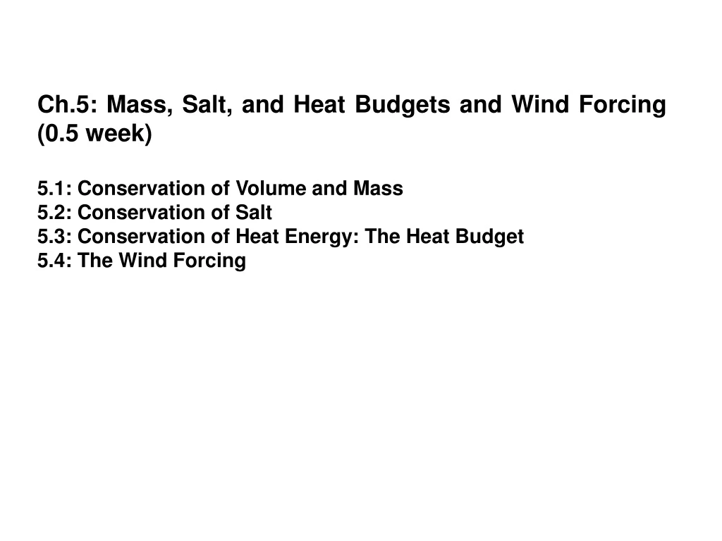
Ch.5: Mass, Salt, and Heat Budgets and Wind Forcing (0.5 week) 5.1: Conservation of Volume and Mass 5.2: Conservation of Salt 5.3: Conservation of Heat Energy: The Heat Budget 5.4: The Wind Forcing. Continuity of mass for a small volume of fluid. By continuity, V o = V i.

E N D
Ch.5: Mass, Salt, and Heat Budgets and Wind Forcing (0.5 week) 5.1: Conservation of Volume and Mass 5.2: Conservation of Salt 5.3: Conservation of Heat Energy: The Heat Budget 5.4: The Wind Forcing
Continuity of mass for a small volume of fluid. By continuity, Vo = Vi. Schematic diagram of basin inflows and outflows for conservation of volume discussion. 5.1: Conservation of Mass and Volume Conservation of Mass Viρi+RρR+AxPρP = Voρo+AxEρE V, R are volume transport in the ocean and river run-off (=velocity*area, in m3/s, 1 Sverdrup=106m3/s , corresponding to a mass transport 109 kg/s), P and E are precipitation and evaporation over an unit area (m/s) and its volume transport should therefore be multiplied by the surface area A. For the ocean, water is almost incompressible and densities are within 3% (between fresh and salty water, or between surface and deep ocean water), so mass conservation becomes Conservation of Volume Vi+R+AxP = Vo+AxE Or Vo-Vi = F where F is the freshwater transport F=(R+AxP)-AxE=R+A(P-E) that is supplied to the region. F>0 positive means net supply, and F<0 a net loss of freshwater. Different from the volume transport V, freshwater transport represents the excess of freshwater in one region relative to another, or it is the convergence/divergence of freshwater (Vo-Vi =F) and is therefore usually much smaller than the volume transport V. In subsurfaceopen ocean, R=P=E=0, So volume conservation becomes Transport conservation Vo-Vi = 0 FIGURE 5.1, 5.2
5.2: Conservation of Salt Near Conservation of Salt: Each year, river inputs dissolved solids of 3x10¹² kg, total dissolved salt in the ocean is 5x10¹⁹ kg. (earth surface A=4*pi*R^2, ocean volume V=Ax4kmx0.7, water weight W=1000kg/m^3 V, Salt S=W*35/1000) Therefore, the salt in the ocean increases each year by a pencentge of 3x10¹²/5x1019=1/17,000,000, that is one part in 17 million. The most accurate measurement has the accuracy of 0.001, assuming mean salinity of 35ppt, this corresponds to 0.001x5x1019/35, which in turn corresponds to one part in 35,000 because 0.001x5x1019/35 /5x1019 = 0.001/35 =1/35000 Since (1/35000)/(1/17,000,000)=17000,000/35,000 = 17,000/35=~ 500 times The measurement accuracy is 500 times larger than the annual salt input from river. If we consider the loss of salt from surface evaporation in evaporites, the increase of salt is even smaller. So, at hundreds of years or even longer time scale, we can consider the total salt is conserved. Salinity Change With the conservation of salt, salinity S can still be changed due to the addition/subtraction of freshwater such as river input, precipitation and evaporation, and melting. In particular, the melting of ice sheet (Greenland is 7-m, Antarctic is 34-m) dilutes ocean salinity. With 1 m global sea level equivalent ice sheet melting, given an ocean depth of 4000m, the global mean salinity will be reduced by 1/4000 which is 4 times smaller than the measurement accuracy. On the other hand, glaciation will lock water on the continent and therefore increase oceanic salinity. At the last glacial maximum, sea level is lowered by 120m, and the salinity is therefore increased by 120m/4000m~1/34, so the total salinity will be increased by about 1 ppt! S/M=34/1000, S/M(1+1/34)=(34*S/35*M)~=33/1000 Global sea level change in the last 100,000 years
Salt and Freshwater Budget Salt Conservation Equation In an enclosed region, since salinity is defined as S=mass of salt/mass of water, the total salinity conservation can be expressed as Salt input flux = ViρiSi = VoρoSo = Salt output flux Since ρi ~ ρo within 3% error (fresh vs salty waters), ViSi = VoSo Salt conservation equation Using the volume conservation equation, Vo-Vi =F, we have Vi=FSo/(Si-So) or Vo=FSi/(Si-So) Knudsen relation 1 This relation shows that the volume transport can be calculated from the freshwater transport F and salinities. Freshwater Transport and Budget Equivalently, if we know the volume transport and salinity, we can calculate the freshwater transport as F=Vi(Si/So-1) or F=Vo(1-So/Si) . Knudsen relation 2 The Knudsen relation 2 calculates the freshwater transport F from volume transport V and salinity. Usually, S are large (close 35) but with a small difference. So F is much smaller than V, i.e. F/V ~ (Si-So)/S <<1, such that a small F can drive a much larger volume transport and in turn faster (volume) flushing time! The freshwater budget is the same as the volume conservation discussed before, Vo-Vi = F, and represents the divergence/convergence of net volume transport. In general for a continuous open ocean, at each point (section), the freshwater transport can be calculated (similar to K relation 2) as F=v(1-S/Sr) around the area boundary, with v as the velocity and Sr as a globally uniform reference salinity. And salt transport as vS. Note (?): The freshwater transport F here is not the true volume freshwater transport: With the total mass as m and salt mass as s (both per unit volume), with the definition of salinity as S=s/m, we have the total volume freshwater transport as V (m-s)= V(m-Sm)=V(1-S)m. With total mass conserved, the volume freshwater budget of an enclosed basin is therefore Vo(1-So)m=F+Vi(1-Si)m freshwater volume budget This is awkward for calculation in practice because we only measure salinity S and volume transport V.
Examples Schematic diagrams of inflow and outflow characteristics for (a) Mediterranean Sea (negative water balance; net evaporation), (b) Black Sea (positive water balance; net runoff/precipitation). Black Sea: Positive Water Balance (net gain of water, AE<AP+R or F>0) Dense inflow of Si=35 psu from Mediterranean through the Strait of Bosporus at the lower layer is balanced by a lighter outflow of So=17 psu. We also measure Vi=0.0095 Sv., Vo=0.019 Sv., so we have F=0.0095 Sv. With this inflow rate, the turnover time for Black Sea is 1000-2000 years. (old, consistent with deep water No O2!) Question: Why Black Sea is so fresh? Mechanism: river run-off and precipitation is so strong that even winter there is no convection, so driven by local wind forcing. Mediterranean Sea: Negative Water Balance (net loss of water, AE>AP+R or F<0) Dense water outflows over the sill of the Strait of Gibraltar, injecting salty water of So=38.4 psu into the N. Atlantic, replaced by inflow in the upper layer of N. Atlantic water of Si=36.1 pus. We also measure Vi=0.72 Sv., so we have Vo=0.68 Sv., and a very small loss of water from surface F=-0.04 Sv. The inflow Vi will take 165 years to fill the basin (residence time). (young, consistent with deep water O2~160 umol/kg) Question: Why Mediterranean is so salty? Mechanism: winter cooling and evaporation leads to convection in the north, driving the flow FIGURE 5.3
Open Ocean (a) Net evaporation and precipitation (E–P) (cm/yr) based on climatological annual mean data(1979–2005) from the National Center for Environmental Prediction. Net precipitation is negative (blue), net evaporation is positive (red). Overlain: freshwater transport divergences (Sverdrups or 1×10⁹ kg/sec) based on ocean velocity and salinity observations. (b) Meridional (south to north) freshwater mass transport (Sverdrups), positive northward, based on ocean velocity and salinity observations (direct) and based on atmospheric analyses (continuous curves). For the world ocean, the ocean gain freshwater in the extratropics (and deep tropics ITCZ) through excessive precipitation (over evaporation) and loss freshwater through evaporation in the subtropics. Therefore, there has to be a freshwater transport in the ocean from the extratropics to the subtropics. (the opposite occurs in the atmosphere: atmospheric moisture transports moisture from the subtropics to the extratropics!) The volume transport is usually large, V ~ 10 to 100 Sv., while the freshwater transport is small, usually ~ 0.1-1 Sv. FIGURE 5.4
Distribution of 100 units of incoming shortwave radiation from the sun to Earth’s atmosphere and surface: long-term world averages. 5.3: Conservation of Heat Energy: the Heat Budget The column heat budget Qt=Qs+Qb+Qh+Qe+Qv Heat storage Qt=Int dz CpρdT/dt Shortwave Qs=(1-α)Qclearsky(1-0.62C+0.0019θNoon) Longwave -Qb=εσSBTw4(0.39-0.05e1/2)(1-kC2)+4εσSBTw3(Tw-TA) Latent heat -Qe=LFe , Fe=ρCeu(qs-qa) Sensible heat -Qh=ρCeChu(Ts-Ta) Heat Transport Qv=-Int dz Cpρ div(vT) FIGURE 5.5
Absorption of shortwave radiation as a function of depth (m) and chlorophyll concentration, C (mg m–3). The vertical axis is depth (m). The horizontal axis is the ratio of the amount of radiation at depth z to the amount of radiation just below the sea surface, at depth “0.” Note that the horizontal axis is a log axis, on which exponential decay would appear as a straight line. Sun glint in the Mediterranean Sea. Shortwave absorption Penetration of up to 100-m, decreases with chlorophyll concentration FIGURE 5.6
Cloud fraction (monthly average for August, 2010) from MODIS on NASA’s Terra satellite. Gray scale ranges from black (no clouds) to white (totally cloudy). Cloud fraction FIGURE 5.8
Outgoing Longwave Radiation (OLR) for Sept. 15–Dec. 13, 2010. This figure can also be found in the color insert. Longwave Absorption in the top 1 mm! Skin temperature (1 mm) Bulk surface temperature (1-m) used in empirical heat flux formula Outgoing Long Wave (through Top of Atmosphere) FIGURE 5.9
Ice-albedo feedback. In the feedback diagram, arrowheads (closed circles) indicate that an increase in one parameter results in an increase (decrease) in the second parameter. The net result is a positive feedback, in which increased sea ice cover results in ocean cooling that then increases the ice cover still more. Sea Ice Effect FIGURE 5.10
Surface Heat Fluxes Shortwave heat flux Qs Longwave (back radiation) heat flux Qb Evaporative (latent) heat flux Qe. Sensible heat flux Qh Annual average heat fluxes (W/m2). (a) Shortwave heat flux Qs. (b) Longwave (back radiation) heat flux Qb. (c) Evaporative (latent) heat flux Qe. (d) Sensible heat flux Qh. Positive (yellows and reds): heat gain by the sea. Negative (blues): heat loss by the sea. Contour intervals are 50 W/m2 in (a) and (c), 25 W/m2 in (b), and 15 W/m2 in (d). Data are from the National Oceanography Centre, Southampton (NOCS) climatology (Grist and Josey, 2003). This figure can also be found in the color insert. FIGURE 5.11
Net Surface Heat Flux Annual average net heat flux (W/m2). Positive: heat gain by the sea. Negative: heat loss by the sea. Data are from the NOCS climatology (Grist and Josey, 2003). Superimposed numbers and arrows are the meridional heat transports (PW) calculated from ocean velocities and temperatures, based on Bryden and Imawaki (2001) and Talley (2003). Positive transports are northward. FIGURE 5.12
Heat input through the sea surface (where 1 PW = 1015 W) (world ocean) for 1º latitude bands for all components of heat flux. Data are from the NOCS climatology (Grist and Josey, 2003). Surface Heat Fluxes Shortwave ~ Latent Heat + Longwave + Sensible FIGURE 5.13
Meridional Heat Transport Methods: Indirect 1 (surface flux for OHT) Indirect 2 (TOP flux minus AHT) Direct Poleward heat transport (W) for the world’s oceans (annual mean). (a) Indirect estimate (light curve) summed from the net air–sea heat fluxes of Figures 5.12 and 5.13. Data are from the NOCS climatology, adjusted for net zero flux in the annual mean. (b) Summary of various direct estimates (points with error bars) and indirect estimates. The direct estimates are based on ocean velocity and temperature measurements. The range of estimates illustrates the overall uncertainty of heat transport calculations. Combined Atmos+Ocean Heat Transport Ocean Heat Transport AHT OHT FIGURE 5.14
Meridional Heat Transport in Individual Oceans Annual average net heat flux (W/m2). Positive: heat gain by the sea. Negative: heat loss by the sea. Data are from the NOCS climatology (Grist and Josey, 2003). Superimposed numbers and arrows are the meridional heat transports (PW) calculated from ocean velocities and temperatures, based on Bryden and Imawaki (2001) and Talley (2003). Positive transports are northward. FIGURE 5.12
Atlantic Meridional Heat Transport T S Atlantic Ocean Pacific Ocean Wust story
Annual mean air–sea buoyancy flux converted to equivalent heat fluxes (W/m2), Positive values indicate that the ocean is becoming less dense. Contour interval is 25 W/m2. Buoyancy Flux =α*Heat Flux + β*Freshwater Flux Buoyancy flux NADW formation cooling Mode water formation Heat flux Freshwater flux cooling FIGURE 5.15
Surface Wind Stress Mean wind stress (arrows) and zonal wind stress (color shading) (N/m2): (a) annual mean, (b) February, and (c) August, from the NCEP reanalysis 1968–1996 (Kalnay et al., 1996). Major components: Trade wind Westerly wind Monsoon wind ITCZ FIGURE 5.16ac
Wind Stress Curl ===> Ekman pumping ===> thermocline circulation (d) Mean wind stress curl based on 25 km resolution QuikSCAT satellite winds (1999–2003). Downward Ekman pumping (Chapter 7) is negative (blues) in the Northern Hemisphere and positive (reds) in the Southern Hemisphere. FIGURE 5.16d
Sverdrup transport Upper ocean, wind-driven transport Sverdrup transport (Sv), where blue is clockwise and positive is counterclockwise circulation. Wind stress data are from the NCEP reanalysis 1968–1996 (Kalnay et al., 1996). FIGURE 5.17