Download
1 / 23
230 likes | 461 Views
Hash Tables. a hash table is an array of size Tsize has index positions 0 .. Tsize-1 two types of hash tables closed hash table array element type is a <key, value> pair all items stored in the array Chained (open) hash table

E N D
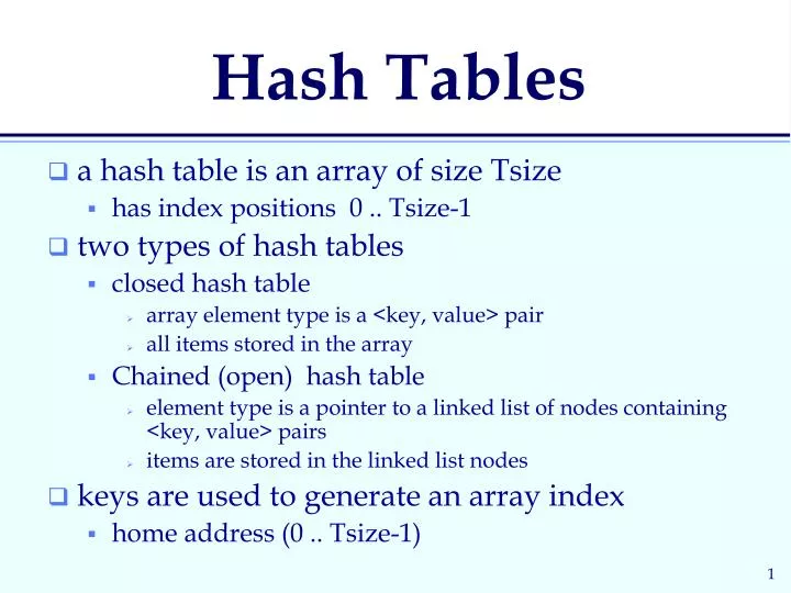
Hash Tables • a hash table is an array of size Tsize • has index positions 0 .. Tsize-1 • two types of hash tables • closed hash table • array element type is a <key, value> pair • all items stored in the array • Chained (open) hash table • element type is a pointer to a linked list of nodes containing <key, value> pairs • items are stored in the linked list nodes • keys are used to generate an array index • home address (0 .. Tsize-1)
faster searching • "balanced" search trees guarantee O(log2 n) search path by controlling height of the search tree • AVL tree • 2-3-4 tree • red-black tree (used by STL associative container classes) • hash table allows for O(1) search performance • search time does not increase as n increases
Considerations • How big an array? • load factor of a hash table is n/Tsize • Hash function to use? • int hash(KeyType key) // 0 .. Tsize-1 • Collision resolution strategy? • hash function is many-to-one
Hash Function • a hash function is used to map a key to an array index (home address) • search starts from here • insert, retrieve, update, delete all start by applying the hash function to the key
Some hash functions • if KeyType is int - key % TSize • if KeyType is a string - convert to an integer and then % Tsize • goals for a hash function • fast to compute • even distribution • cannot guarantee no collisions unless all key values are known in advance
An Closed Hash Table Hash (key) produces an index in the range 0 to 6. That index is the “home address” 0 1 2 3 4 5 6 K3 K3info K1 K1info Some insertions: K1 --> 3 K2 --> 5 K3 --> 2 K2 K2info key value
Handling Collisions 0 1 2 3 4 5 6 K6 K6info Some more insertions: K4 --> 3 K5 --> 2 K6 --> 4 K3 K3info K1 K1info K4 K4info K2 K2info Linear probing collision resolution strategy K5 K5info
Search Performance Average number of probes needed to retrieve the value with key K? 0 1 2 3 4 5 6 K6 K6info K hash(K) #probes K1 3 1 K2 5 1 K3 2 1 K4 3 2 K5 2 5 K6 4 4 K3 K3info K1 K1info K4 K4info K2 K2info 14/6 = 2.33 (successful) K5 K5info unsuccessful search?
K3 K3info K5 K5info K1 K1info K4 K4info K6 K6info K2 K2info linked lists of synonyms A Chained Hash Table 0 1 2 3 4 5 6 insert keys: K1 --> 3 K2 --> 5 K3 --> 2 K4 --> 3 K5 --> 2 K6 --> 4
0 1 2 3 4 5 6 K3 K3info K5 K5info K1 K1info K4 K4info K6 K6info K2 K2info Search Performance Average number of probes needed to retrieve the value with key K? K hash(K) #probes K1 3 1 K2 5 1 K3 2 1 K4 3 2 K5 2 2 K6 4 1 8/6 = 1.33 (successful) unsuccessful search?
successful search performance open addressing open addressing chaining (linear probing) (double hashing) load factor 0.5 1.50 1.39 1.25 0.7 2.17 1.72 1.35 0.9 5.50 2.56 1.45 1.0 ---- ---- 1.50 2.0 ---- ---- 2.00
Factors affecting Search Performance • quality of hash function • how uniform? • depends on actual data • collision resolution strategy used • load factor of the HashTable • N/Tsize • the lower the load factor the better the search performance
Traversal • Visit each item in the hash table • Closed hash table • O(Tsize) to visit all n items • Tsize is larger than n • Chained hash table • O(Tsize + n) to visit all n items • Items are not visited in order of key value
Deletions? • search for item to be deleted • chained hash table • find node and delete it • open hash table • must mark vacated spot as “deleted” • is different than “never used”
Hash Table Summary • search speed depends on load factor and quality of hash function • should be less than .75 for open addressing • can be more than 1 for chaining • items not kept sorted by key • very good for fast access to unordered data with known upper bound • to pick a good TSize
heap • is a binary tree that • is complete • has the heap-order property • max heap - item stored in each node has a key/priority that is >= the priority of the items stored in each of its children • min heap - item stored in each node has a key/priority that is <= the priority of the items stored in each of its children • efficient data structure for PriorityQueue ADT • requires the ability to compare items based on their priorities • basis for the heapsort algorithm
23 18 9 8 12 7 1 4 2 1 4 2 9 8 7 18 23 12 two heaps A heap is always a complete binary tree
23 18 9 8 12 7 1 4 2 A Size 23 18 9 8 12 7 1 4 2 0 1 2 3 4 5 6 7 8 9 a complete binary tree can be stored in an array for the item in A[i]: leftChild is in A[2i+1] rightChild is in A[2i+2] parent is in A[(i-1)/2]
PriorityQueue ADT • Data Items • a collection of items which can be ordered by priority • Operations • constructor - creates an empty PQ • empty () - returns true iff a PQ is empty • size () - returns the number of items in a PQ • push (item) - adds an item to a PQ • top () - returns the item in a PQ with the highest priority • pop () – removes the item with the highest priority from a PQ
PQ Data structures • unordered array or linked list • push is O(1) • top and pop are (n) • ordered array or linked list • push is O(n) • top and pop are (1) • heap • top is O(1) • push and pop are O(log2 n) • STL has a priority_queue class • is implemented using a heap
PQ operations • top • return item at A[0] • push and pop must maintain heap-order property • push • put new item at end (in A[size]) • re-establish the heap-order property by moving the new item to where it belongs • pop • A[0] is item to delete • swap A[0] and A[size-1] • move item at A[0] down a path to where it belongs
23 18 9 8 12 7 1 4 2 18 12 9 8 2 7 1 4 18 12 2 23 A Size 23 18 9 8 12 7 1 4 2 8 0 1 2 3 4 5 6 7 8 9 pop( )
Balanced Search Trees • several varieties (Ch.13) • AVL trees • 2-3-4 trees • Red-Black trees • B-Trees (used for searching secondary memory) • nodes are added and deleted so that the height of the tree is kept under control • insert and delete take more work, but retrieval (also insert & delete) never more than log2 n because height is controlled