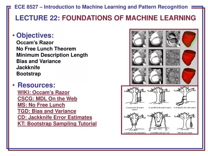
LECTURE 22: FOUNDATIONS OF MACHINE LEARNING

1. LECTURE 22: FOUNDATIONS OF MACHINE LEARNING • Objectives:Occam’s RazorNo Free Lunch TheoremMinimum Description LengthBias and VarianceJackknifeBootstrap • Resources:WIKI: Occam's RazorCSCG: MDL On the WebMS: No Free LunchTGD: Bias and VarianceCD: Jackknife Error EstimatesKT: Bootstrap Sampling Tutorial

2. No Free Lunch Theorem • A natural measure of generalization is the expected value of the error given D: • where δ() denotes the Kronecker delta function (value of 1 if the two arguments match, a value of zero otherwise). • The expected off-training set classification error when the true function F(x) and the probability for the kth candidate learning algorithm is Pk(h(x)|D) is: • No Free Lunch Theorem: For any two learning algorithms P1(h|D) and P2(h|D), the following are true independent of the sampling distributionP(x) and the number of training points: • Uniformly averaged over all target functions, F, E1(E|F,n) – E2(E|F,n) = 0. • For any fixed training set D, uniformly averaged over F, E1(E|F,n) – E2(E|F,n) = 0. • Uniformly averaged over all priors P(F), E1(E|F,n) – E2(E|F,n) = 0. • For any fixed training set D, uniformly averaged over P(F), E1(E|F,n) – E2(E|F,n) = 0.

3. Analysis • The first proposition states that uniformly averaged over all target functions the expected test set error for all learning algorithms is the same: • Stated more generally, there are noiand j such that for all F(x),Ei(E|F,n) > Ej(E|F,n). • Further, no matter what algorithm we use, there is at least one target function for which random guessing Is better. • The second proposition states that even if we know D, then averaged over all target functions, no learning algorithm yields a test set error that is superior to any other: • The six squares represent all possibleclassification problems. If a learningsystem performs well over some setof problems (better than average), it must perform worse than averageelsewhere.

4. Algorithmic Complexity • Can we find some irreducible representation of all members of a category? • Algorithmic complexity, also known as Kolmogorov complexity, seeks to measure the inherent complexity of a binary string. • If the sender and receiver agree on a mapping, or compression technique, the pattern x can be transmitted as y and recovered as x=L(y). • The cost of transmission is the length of y,|y|. • The least such cost is the minimum length and denoted: • A universal description should be independent of the specification (e.g., the programming language or machine assembly language). • The Kolmogorov complexity of a binary string x, denoted K(x), is defined as the size of the shortest program string y, that, without additional data, computes the string x: • where U represents an abstract universal Turing machine. • Consider a string of n 1s. If our machine is a loop that prints 1s, we only need log2n bits to specify the number of iterations. Hence, K(x) = O(log2n).

5. Minimum Description Length (MDL) • We seek to design a classifier that minimizes the sum of the model’s algorithmic complexity and the description of the training data, D, with respect to that model: • Examples of MDL include: • Measuring the complexity of a decision tree in terms of the number of nodes. • Measuring the complexity of an HMM in terms of the number of states. • We can view MDL from a Bayesian perspective: • The optimal hypothesis, h*, is the one yielding the highest posterior: • Shannon’s optimal coding theorem provides a link between MDL and Bayesian methods by stating that the lower bound on the cost of transmitting a string x is proportional to log2P(x).

6. Bias and Variance • Two ways to measure the match of alignment of the learning algorithm to the classification problem involve the bias and variance. • Bias measures the accuracy in terms of the distance from the true value of a parameter – high bias implies a poor match. • Variance measures the precision of a match in terms of the squared distance from the true value – high variance implies a weak match. • For mean-square error, bias and variance are related. • Consider these in the context of modeling data using regression analysis. Suppose there is an unknown function F(x) which we seek to estimate based on n samples in a set D drawn from F(x). • The regression function will be denoted g(x;D). The mean square error of this estimate is (see lecture 5, slide 12): • The first term is the bias and the second term is the variance. • This is known as the bias-variance tradeoff since more flexible classifiers tend to have lower bias but higher variance.

7. Bias and Variance For Classification • Consider our two-category classification problem: • Consider a discriminant function: • Where ε is a zero-mean random variable with a binomial distribution with variance: • The target function can be expressed as . • Our goal is to minimize . • Assuming equal priors, the classification error rate can be shown to be: • where yB is the Bayes discriminant (1/2 in the case of equal priors). • The key point here is that the classification error is linearly proportional to , which can be considered a boundary error in that it represents the incorrect estimation of the optimal (Bayes) boundary.

8. Bias and Variance For Classification (Cont.) • If we assume p(g(x;D)) is a Gaussian distribution, we can compute this error by integrating the tails of the distribution (see the derivation of P(E) in Chapter 2). We can show: • The key point here is that the first term in the argument is the boundary bias and the second term is the variance. • Hence, we see that the bias and variance are related in a nonlinear manner. • For classification the relationship is multiplicative. Typically, variance dominates bias and hence classifiers are designed to minimize variance. • See Fig. 9.5 in the textbook for an example of how bias and variance interact for a two-category problem.

9. Resampling For Estimating Statistics • How can we estimate the bias and variance from real data? • Suppose we have a set D of n data points, xi for i=1,…,n. • The estimates of the mean/sample variance are: • Suppose we wanted to estimate other statistics, such as the median or mode. There is no straightforward way to measure the error. • Jackknife and Bootstrap techniques are two of the most popular resampling techniques to estimate such statistics. • Use the “leave-one-out” method: • This is just the sample average if the ith point is deleted. • The jackknife estimate of the mean is defined as: • The variance of this estimate is: • The benefit of this expression is that it can be applied to any statistic.

10. Jackknife Bias and Variance Estimates • We can write a general estimate for the bias as: • The jackknife method can be used to estimate this bias. The procedure is to delete points xi one at a time from D and then compute: . • The jackknife estimate is: • We can rearrange terms: • This is an unbiased estimate of the bias. • Recall the traditional variance: • The jackknife estimate of the variance is: • This same strategy can be applied to estimation of other statistics.

11. Bootstrap • A bootstrap data set is one created by randomly selecting n points from the training set D, with replacement. • In bootstrap estimation, this selection process is repeated B times to yield B bootstrap data sets, which are treated as independent sets. • The bootstrap estimate of a statistic, , is denoted and is merely the mean of the B estimates on the individual bootstrap data sets: • The bootstrap estimate of the bias is: • The bootstrap estimate of the variance is: • The bootstrap estimate of the variance of the mean can be shown to approach the traditional variance of the mean as . • The larger the number of bootstrap samples, the better the estimate.

12. Summary • Analyzed the No Free Lunch Theorem. • Introduced Minimum Description Length. • Discussed bias and variance using regression as an example. • Introduced a class of methods based on resampling to estimate statistics. • Introduced the Jackknife and Bootstrap methods. • Next: Introduce similar techniques for classifier design.