Download
1 / 22
230 likes | 422 Views
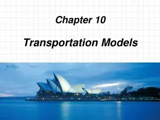
Bus 480 – Lecture 2 Transportation and Assignment models. Transportation Model. Product is transported from location to location minimum cost Each source able to supply a fixed number of units Each destination has a demand for a fixed number of units

E N D
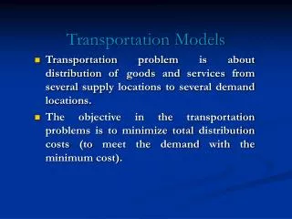
Transportation Model • Product is transported from location to location minimum cost • Each source able to supply a fixed number of units • Each destination has a demand for a fixed number of units • Can have multiple solutions, but the same minimum cost
Transportation Model • Let Xij = amount of product from point i to point j • We will minimize cost • The constraints will be the amount that is shipped out of point i to point j • Supply Constraints • Demand Constraints • Each row will be its own constraint • Each column will be its own constraint
Example #4 • Each cell represents the cost of shipping one unit from site i to site j • The cost of sending one unit of product from site A to site 1 is $6 • Site 1 has a demand of 80 units • Site A can supply 130 units
Example #4 Let XA1=amount shipped from site A to site 1 XA2=amount shipped from site A to site 2 XA3=amount shipped from site A to site 3 XB1=amount shipped from site B to site 1 XB2=amount shipped from site B to site 2 XB3=amount shipped from site B to site 3 XC1=amount shipped from site C to site 1 XC2=amount shipped from site C to site 2 XC3=amount shipped from site C to site 3
Demand/Supply Check • Check to see if total supply equals total demand. • If yes, then constraints are equality • If no, then if supply > demand then supply constraints are <= and demand is = • if supply < demand then supply constraints are = and demand is <=
Example 4 • Total demand : 80 + 110 + 60 = 250 • Total supply : 130 + 70 + 100 = 300 • Supply is greater than demand. • Cannot ship more product than is demanded • Supply constraints will be <= • Can meet all the demand • Demand constraints will be =
Example 4 • Objective Function • Min 6XA1 + 9XA2 + 11XA3 + 12XB1 + 3XB2 + 5XB3 + 4XC1 + 8XC2 + 11XC3 • Note the structure. It’s the same as the table
Example 4 • Supply Constraints XA1 + XA2 + XA3 ≤ 130 XB1 + XB2 + XB3 ≤ 70 XC1 + XC2 + XC3 ≤ 100 Why are the signs ≤ ? • Demand Constraints XA1 + XB1 + XC1 = 80 XA2 + XB2 + XC2 = 110 XA3 + XB3 + XC3 = 60 Why are the signs =?
Example 4 Hint : Copy the table twice. Once for the decision variables and one for costs Each row will be a sum. Each column will be a sum. Objective function will be sumproduct
Example 4 - Solution Site A : Ship 80 units to site 2 Site B : Ship 10 units to site 2 and 60 units to site 3 Site C : Ship 80 units to site 1 and 20 units to site 2 Minimum cost = $1530 Check All constraints to verify the results
Transshipment Problems • Have intermediate sites • If an intermediate site cannot hold product then everything going into the site must equal that going out of the site • Still have supply and demand constraints • One extra constraint for each site
A F D B G E C H Transshipment Diagram • Site D and E are intermediary Sites • Sites A, B, C are supply sites • Sites F, G, H are demand sites
Transshipment Constraints • Everything going into site d must equal everything leaving site d Xad + Xbd + Xcd = Xdf + Xdg + Xdh • In Excel, move all variables to the left side of the equation Xad + Xbd + Xcd - Xdf - Xdg - Xdh = 0
Example 41 • Ship from European port to US port • Once product gets to US port, it is immediately shipped to the inland port • This makes the transshipment constraints=0 • If the port can hold product, then 0 will change to the amount of product the port can hold, typically ≤ . Why?
Example 41- Solution Cost function is the addition of multiple sumproducts
Assignment Problem • Set up identical the transportation problem • All constraints are equal to 1 • Xij will be binary = 1 if selected, 0 otherwise