Download
1 / 79
800 likes | 1k Views
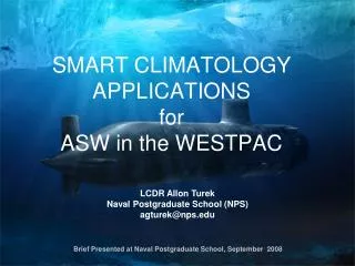
Smart Climatology for ASW: Initial Assessments and Recommendations. Tom Murphree Naval Postgraduate School (NPS) murphree@nps.edu Bruce Ford Clear Science, Inc. (CSI) bruce@clearscienceinc.com Brief Presented to CAPT Jim Berdeguez, USN CNMOC 14 August 2007.

E N D
Smart Climatology for ASW: Initial Assessments and Recommendations Tom Murphree Naval Postgraduate School (NPS) murphree@nps.edu Bruce Ford Clear Science, Inc. (CSI) bruce@clearscienceinc.com Brief Presented to CAPT Jim Berdeguez, USN CNMOC 14 August 2007 ASW Smart Climo, Aug 07, murphree@nps.edu
Smart Climatology for ASW Outline of This Brief SlidesTopic 3-8 Overview 9-14 Background Definitions and Concepts 15-19 Data and Methods Initial Assessments: 20-23 a. Atmospheric Variables 24-35 b.Ocean Temperature 35-42 c. Ocean Salinity 43-47 d.Sea Surface Heights and Currents 48-54 Preliminary Findings 55-60 Recommendations and Proposals 61 Contact Information 62-79 Back-Up Slides ASW Smart Climo, Aug 07, murphree@nps.edu
Smart Climatology for ASW Slides 3-8: Overview ASW Smart Climo, Aug 07, murphree@nps.edu
Acknowledgements • Dennis Krynen of NAVO for providing GDEM and other Navy climatological datasets, and much useful discussion • ASW RBC staff for providing insights into importance of atmospheric and oceanic climatology in providing METOC support for ASW • Students in the NPS climatology courses, and NPS thesis research students, for many useful discussions and tests of the operational applications of smart climatology ASW Smart Climo, Aug 07, murphree@nps.edu
NPS Smart Climatology Program The NPS Smart Climatology program has four main components: 1. Education 2. Basic and Applied Research 3. Prototype Operational Product Development 4. Product Transitioning For more information, including our major R&D reports from 2000 to present, see: http://wx.met.nps.navy.mil/smart-climo/. Materials for the NPS Modern Climatology and Advanced Climatology courses are available on request. Note: The RTP smart climatology project is not affiliated with the NPS Smart Climatology program. ASW Smart Climo, Aug 07, murphree@nps.edu
Motivation for Improving Navy Atmospheric and Oceanic Climatology • Prior assessments have shown that DoD, and specifically Navy, climatology lags significantly behind the state of the science, and the gap is widening. • Improved, at-your-fingertips, smart climatology has the potential to significantly improve the situational awareness of METOC personnel, and the quality of all METOC products --- “A rising tide lifts all ships.” • Existing civilian ocean reanalysis products provide very good 4-D climatological representations of the atmosphere and ocean. • Greatly improved and much higher resolution civilian coupled atmosphere-ocean reanalysis products are scheduled for release in FY08-FY09. • The potential exists to develop state-of-the-science climatological visualization, analysis, forecasting, and training tools at a relatively low cost. ASW Smart Climo, Aug 07, murphree@nps.edu
Purpose of This Initial Study • At request of CAPT Jim Berdeguez, develop prototype smart climatology products for ASW. • Compare Navy atmospheric and oceanic climatologies to climatologies based on existing civilian atmospheric and oceanic reanalysis data sets. • Assess value of providing state-of-the-science ocean climatologies for planning and execution of ASW operations. • Make recommendations for how to proceed with providing climatological support for ASW operations. ASW Smart Climo, Aug 07, murphree@nps.edu
Objectives of This Initial Study • Use existing, long term ,civilian, ocean reanalysis data to prepare, analyze, and display long term mean (LTM) surface and subsurface ocean fields. • Assess ability of reanalysis data to represent LTM oceanic patterns and processes important in ASW. • Conduct initial comparisons of oceanic and atmospheric based on existing civilian sector reanalyses and on existing Navy climatologies • Focus region and time: VS07 region, August long term mean conditions • Note: no consideration in this initial study of climate regimes and • variations, such as high wind stress and low wind stress regimes, El Nino / La Nina, Madden-Julian Oscillation, etc. ASW Smart Climo, Aug 07, murphree@nps.edu
Smart Climatology for ASW Slides 9-14: Background Definitions and Concepts ASW Smart Climo, Aug 07, murphree@nps.edu
Background Definitions and Concepts – Section 1 • Climate– Expected state of the environment based on scientific observations, analyses, theories, and models, and is not limited to just observational analyses. Expected state accounts for long term means and variations from these means that occur over long periods (e.g., anomalous trends and oscillations that occur over weeks, years, or longer). • Smart Climatology– Climatology applied to military uses that employs all relevant tools of modern climatology, such as: • Full suite of in situ and remote observational data sets • Reanalysis • Downscaling • Data access, mining, and processing tools • Modern statistical and dynamical analysis methods • Long term means and higher order statistics • Climate variations (e.g., regimes, trends, oscillations) • Climate system monitoring • Climate system modeling • Statistical and dynamical climate forecasting • Online, real-time, user-driven, data access, analysis, and display Smart Climatology State-of-the-science basic and applied climatology that directly supports DoD operations ASW Smart Climo, Aug 07, murphree@nps.edu 10
Background Definitions and Concepts – Section 2 Reanalysis- The analysis of climate system components using modern analysis processes to analyze past and present states of the climate system. Reanalysis is the same as standard atmospheric or oceanic analysis, except that it applies a consistent set of analysis procedures to all times in the reanalysis period. Oceanic and atmospheric reanalyses yield gridded data sets that are temporally and spatially continuous (i.e., no temporal or spatial gaps). For many reanalyses, the reanalysis period is several decades long, and the reanalysis region is the global ocean or atmosphere. Reanalyses can have relatively high temporal and spatial resolution (e.g., mesoscale reanalyses: hourly and 10 km; global reanalyses: six hourly and one degree). Reanalysis fields are a major source of climate information since they fill in the spatial and temporal gaps in climatologies based strictly on observations. Traditional observational climatologies either leave these gaps unfilled or use statistical methods (e.g., interpolation, correlation) techniques to fill in these gaps. Reanalyses use state-of-the-science data assimilation and oceanic and/or atmospheric models to fill in these gaps, and develop a dynamically balanced description of the climate system. Reanalysis data include many derived fields (momentum, energy, and mass fluxes; sea surface heights; currents; precipitation; soil moisture, etc.) for which direct observations may be difficult to obtain. ASW Smart Climo, Aug 07, murphree@nps.edu 11
Background Definitions and Concepts – Section 3 Evaluating Reanalyses - Several organizations have produced and are producing reanalyses of the atmosphere and ocean for use in basic and applied climatology (e.g., NOAA, ECMWF, NASA, AFCCC, NRL, universities). But there can be large differences between reanalyses in terms of their data and methods, temporal and spatial coverage, quality control procedures, verification, and accuracy. The net result is that some reanalyses are much more useful and reliable than others, and some reanalyses should be used with a fair bit of caution. These differences among reanalyses reflect the complexity and high cost of developing an extensive and high quality reanalysis. ASW Smart Climo, Aug 07, murphree@nps.edu 12
Background Definitions and Concepts – Section 4 Long Term Mean (LTM)- The mean of many observations collected over a long period of time (the base period). The standard period for calculating a LTM is 30 years. LTMs are commonly based on observations made at the same location and same time of day but at many different dates (e.g., T at 00Z on 01 January of 30 consecutive years). LTMs are common and very useful quantities in climatology. But LTMs do not represent many important temporal and spatial aspects of the climate system, such as climate variation trends and oscillations. These are better represented by other types of means and by higher order statistical quantities (e.g., select composite means, variance, standard deviation, temporal clusters, principal components). ASW Smart Climo, Aug 07, murphree@nps.edu 13
Background Definitions and Concepts – Section 5 • Methods for Generating Climatologies • 1. Observations • Average all available observations for a given location and time of year. • Pros: Based strictly on observations, with no influence of statistical or dynamical methods for filling in temporal and spatial data gaps. • Cons: In data sparse regions (e.g., most of the ocean), there can be major data gaps. • 2. Observations with statistically-based filling of gaps • Use all available observations with data gaps filled via statistical methods (e.g., interpolation, correlation). Relies, in effect, on statistical model to fill in gaps. ManyNavy operational climatologiesgenerated using this method. • Pros: Relies on observations alone to develop statistical tools for filling gaps • Cons: Limited by the number of observations and the number of observed variables, especially in data sparse regions. No explicit check for dynamic consistency. • Observations with reanalysis-based filling of gaps • Uses all available observations with data gaps filled by data assimilation and dynamical models. This method used by many state-of-the-artcivilian operational climatologies. Reanalysis climatologies shown in this initial study use this method. • Pros: Data assimilation and dynamical models are well tested and yield dynamically balanced results. • Cons: In data sparse regions, results are strongly dependent on model. ASW Smart Climo, Aug 07, murphree@nps.edu 14
Smart Climatology for ASW Slides 15-19: Data and Methods ASW Smart Climo, Aug 07, murphree@nps.edu
Initial Demonstration Case – Section 1 Oceanic Reanalysis Data Set Used: Simple Ocean Data Assimilation (SODA), version 1.4.2: - Spatial coverage: ~global (0-360E, 75.25S-89.25N) - Temporal coverage: 1958-2001, 44 years - Horizontal resolution: variable but ~ 0.3 x 0.3 degrees * - Vertical resolution: 40 levels, from 5 m to 5374 m 10 levels in the upper 100 m 20 levels in the upper 500 m - Observational input variables: surface winds, T, S - Reanalyzed output variables: x, y, SSH, T, S, u, v - Model similar to z level models used by multiple researchers (e.g., Semtner and Chervin) - Data analyzed: 528 individual monthly means, Jan58–Dec01 horiz res: 0.5 x 0.5 degrees all levels, but focus on upper 500 m base period for calcualting LTMs: 1968-1996 * See notes ASW Smart Climo, Aug 07, murphree@nps.edu
Initial Demonstration Case – Section 2 Atmospheric Reanalysis Data Set Used: NCEP Global Atmospheric Reanalysis: Temporal resolution: six hours; spatial resolution: 2.5 x 2.5 degrees. Available at all standard tropospheric and stratospheric levels. Available from Jan 1948 – present. Provides all standard atmospheric variables, and many less standard ones. Available at menu driven data downlaod, analysis, and display sites provided by NOAA. Note: NCEP global coupled atmospheric-oceanic reanalysis to be available in FY08-FY09, at 0.25 x 0.25 degree resolution in atmosphere, 0.5 x 0.5 degree resolution in ocean. ASW Smart Climo, Aug 07, murphree@nps.edu
Initial Demonstration Case – Section 3 Navy Climatology Data Sets Used: Ocean: Generalized Digital Environmental Model(GDEM), as provided on CD by Dennis Krynen of NAVO. Provides only long term mean values based on data from many decades but especially from most recent decades. Temporal resolution: one month; spatial resolution: 1 x 1 degrees. Variables available: T, S, SVP. Based on observations and statistical interpolation methods to fill gaps. Atmosphere: Surface Marine Gridded Clmatology (SMGC) Version 2.0, as provided in the environmental background section of the VS07 page at the Navy Oceanography Portal on the SIPRnet. Spatial resolution: temporal resolution: one month; spatial resolution: 1 x 1 degrees. Based on observations and statistical interpolation methods to fill gaps. Alternate Navy atmospheric climatology for future investigation: Global Marine Climatic Atlas (GMCA), V. 2.0. For further details on SMGC and GMCA, see: https://navy.ncdc.noaa.gov/marine-servlet/marinegridded.html https://navy.ncdc.noaa.gov/private/products/fleet/gmca.html ASW Smart Climo, Aug 07, murphree@nps.edu
Initial Demonstration Case – Section 4 VS07 Region Plus: 135E-160E, 5N-20N VS07 Period: August ASW Smart Climo, Aug 07, murphree@nps.edu
Smart Climatology for ASW Slides 20-23: Initial Assessments a. Atmospheric Variables ASW Smart Climo, Aug 07, murphree@nps.edu
LTM Surface Wind Stress, August, From Reanalysis August LTM Wind Stress Magnitude and Direction (Base Period 1968-1996) N Pacific High Monsoon Trough E-erly trades SW-erly trades ITCZ N/m2 Note implied relationships between LTM patterns for wind stress and the LTM patterns for, and variability of (and uncertainty in), atmospheric convection, clouds, wind driven mixing, forcing of surface and internal ocean waves, MLD, SLD, BLG, atmospheric EDH, atmospheric EM propagation, etc. There are very large differences between the LTM winds associated with these stresses and the SMGC 2.0 winds provided for VS07 (not shown but available at VS07 page of Navy Oceanography Portal). From SODA oceanic reanalysis ASW Smart Climo, Aug 07, murphree@nps.edu
LTM Precipitation Rate, August, From Reanalysis mm/day Note high precipitation in monsoon trough and ITCZ. Prior studies have shown that precipitation in this region can have a significant impact on upper ocean structure (e.g., formation of low salinity and high temperature layers in upper few meters), which may then impact SVPs, SLDs, and other upper ocean acoustic features. Precipitation is not available from SMGC or GMCA. From NCEP atmospheric reanalysis ASW Smart Climo, Aug 07, murphree@nps.edu
W/m2 LTM Outgoing Longwave Radiation (OLR), August, From Reanalysis OLR is a very useful proxy indicator of clouds and associated winds, surface heat fluxes, and precipitation (e.g., low insolation and high surface winds associated with deep tropical convection), and thus has implications for estimating surface forcing of the ocean and potential impacts on SLD and other ASW-relevant oceanic variables. Blue (red) indicates deep atmospheric convection, high precipitation (clear skies, low precipitation). Low (high) OLR indicates longwave radiation from relatively cold (warm) surface. In tropics, lowest OLR values indicate deep convection, with low amounts of longwave radiation from high cold cloud tops; while highest values indicate clear sky conditions and longwave radiation from relatively warm surfaces (e.g., sea surface). OLR not available from SMGC or GMCA. 23 From NCEP atmospheric reanalysis ASW Smart Climo, Aug 07, murphree@nps.edu
Smart Climatology for ASW Slides 24-35: Initial Assessments b. Ocean Temperature ASW Smart Climo, Aug 07, murphree@nps.edu
LTM Temperature at 5 m, August, From Reanalysis oC • T ranges from low 29s to high 29s. • Warmest water roughly coincident with surface wind convergence zones (monsoon trough, ITCZ). • See also slides 63-64 in Back-Up Slides section. From SODA oceanic reanalysis ASW Smart Climo, Aug 07, murphree@nps.edu
LTM Temperature at 4 m, August, from GDEM .0 oC • Comparisons of reanalysis T at 5 m and GDEM T at 4 m show: • GDEM cooler by ~0.5oC. This is a surprisingly large difference, since near-surface T is relatively well observed. Cooler GDEM due to efforts in development of GDEM to accentuate ML? • GDEM has more small scale structure (e.g., bulls eyes, patchy patterns). Result of GDEM • statistical methods used to fill in gaps? • See also slides 63-64 in Back-Up Slides section. ASW Smart Climo, Aug 07, murphree@nps.edu
LTM Temperature and Currents at 96 m, August, From Reanalysis oC • Warm water at ~11-18N associated with: • - Deep main thermocline • - W-ward transport of relatively warm water by NECC (see back-up slide) • T structures strongly associated with meridional shear in wind stress. From SODA oceanic reanalysis ASW Smart Climo, Aug 07, murphree@nps.edu
LTM Temperature and Currents at 96 m, August, From GDEM oC • Comparisons of T from reanalysis at 96 m and GDEM at 95 m show: • Overall patterns similar. • GDEM cooler than reanalysis, but difference much smaller than near surface. • GDEM has more small scale structure. Result of GDEM statistical methods used to fill in gaps? ASW Smart Climo, Aug 07, murphree@nps.edu
LTM Temperature Along 12N, August, From Reanalysis CI = 1.0 oC • Near-surface isothermal layer in upper 10-25 m. • Small zonal variations. • Main thermocline depth: 150-250 m. From SODA oceanic reanalysis ASW Smart Climo, Aug 07, murphree@nps.edu
LTM Temperature Along 12N, August, From GDEM CI = 1.0 oC • Comparisons of T from reanalysis and GDEM show: • Overall patterns similar, but reanalysis warmer than GDEM in upper 30 m. • GDEM near-surface isothermal layer deeper by ~10-35 m. Due to efforts in development of GDEM to accentuate ML? • GDEM has more fine scale structure. Result of GDEM statistical methods used to fill in gaps? ASW Smart Climo, Aug 07, murphree@nps.edu
LTM Temperature Along 140E, August, From Reanalysis CI = 1.0 oC • Near-surface isothermal layer in upper 10-25 m. • Large meridional variations. • Main thermocline depth: 125-150 m at 5-10N; 150-250 m at 10-15N; 50-100 m at 15-20N. • Thermal structure consistent with velocity structure (see prior and subsequent slides). From SODA oceanic reanalysis ASW Smart Climo, Aug 07, murphree@nps.edu
LTM Temperature Along 140E, August, From GDEM CI = 1.0 oC • Comparisons of T from reanalysis and GDEM show: • Overall patterns similar, but reanalysis warmer than GDEM, especially near surface. • GDEM near-surface isothermal layer deeper by ~10-35 m. Due to efforts in development of GDEM to accentuate ML? • GDEM has more fine scale structure. Result of GDEM statistical methods used to fill in gaps? ASW Smart Climo, Aug 07, murphree@nps.edu
LTM Temperature Profiles, August, From Reanalyses ASW Smart Climo, Aug 07, murphree@nps.edu 33 From SODA oceanic reanalysis
LTM Temperature Profiles, August, From GDEM Reanalysis up to 0.5oC warmer than GDEM in upper 30 m, with largest differences closest to surface. Surprisingly large difference, since near-surface T is relatively well known. Is this due to efforts in development of GDEM to accentuate ML?This difference would lead to deeper SLD in GDEM than in reanalysis. ASW Smart Climo, Aug 07, murphree@nps.edu ASW Smart Climo, Aug 07, murphree@nps.edu
Hypothesized Temperature Profiles, August Schematic T Profiles for Two Hypothesized Regimes, and for LTM of the Two Regimes Hypothesized Regime 1: Occurs during and soon after periods of high insolation and low winds (clear skies). May be enhanced if immediately preceded by high precipitation (e.g., surface freshening). Leads to shallower SLD. Regime 1 Profile Regime 2 Profile LTM of Regime 1 and 2 Profiles Hypothesized Regime 2: Occurs during and soon after periods of low insolation and high winds (e.g., deep convection with strong winds). May be enhanced if immediately preceded by high insolation, low-moderate winds (e.g., high evaporation, salinification). Leads to deeper SLD. If hypothesized profiles are common occurrences (and they probably are), then: (1) the reanalysis T profiles (shown in prior slide and similar to LTM profile in this slide) are probably realistic LTM profiles; and (2) the GDEM profiles (see prior slide) are probably not realistic LTM profiles, although they may be good depictions of Regime 2 conditions. This hypothesis can be tested using regime-based conditional climatologies developed from atmospheric and oceanic reanalyses (e.g., separate climatologies for high and low wind regimes). If a LTM represents opposing regimes, then two or more conditional climatologies may be more useful than a single LTM climatology. The high temporal resolution of reanalyses greatly facilitates development of such conditional climatologies. ASW Smart Climo, Aug 07, murphree@nps.edu
Smart Climatology for ASW Slides 36-42: Initial Assessments c. Ocean Salinity ASW Smart Climo, Aug 07, murphree@nps.edu
LTM Salinity at 5 m, August, From Reanalysis ppt • High S in subtropical areas of high wind speed, low precipitation. • Lower S in tropical areas of lower wind speed, higher precipitation. From SODA oceanic reanalysis ASW Smart Climo, Aug 07, murphree@nps.edu
LTM Salinity at 4 m, August, From GDEM ppt • Comparisons of S from reanalysis at 5 m and GDEM at 4 m show: • Overall patterns similar, but GDEM has greater S range. • In many areas, GDEM saltier or fresher by up to 0.5 ppt. • GDEM has more small scale structure. Result of GDEM statistical methods used to fill in gaps? ASW Smart Climo, Aug 07, murphree@nps.edu
LTM Salinity at 96 m, August, From Reanalysis ppt • Overall patterns similar to those at 5 m, but S ~0.5 ppt higher than at 5 m. From SODA oceanic reanalysis ASW Smart Climo, Aug 07, murphree@nps.edu
LTM Salinity at 95 m, August, From GDEM ppt • Comparisons of S from reanalysis at 96 m and GDEM at 95 m show: • Overall patterns similar, but GDEM has greater S range. • In many areas, GDEM saltier or fresher by ~0.1-0.2 ppt. • GDEM has more small scale structure. Result of GDEM statistical methods used to fill in gaps? ASW Smart Climo, Aug 07, murphree@nps.edu
LTM Salinity Profiles, August, From Reanalyses ASW Smart Climo, Aug 07, murphree@nps.edu 41 From SODA oceanic reanalysis
LTM Salinity Profiles, August, From GDEM GDEM has broader range of S values, especially in upper 70 m. ASW Smart Climo, Aug 07, murphree@nps.edu ASW Smart Climo, Aug 07, murphree@nps.edu
Smart Climatology for ASW Slides 43-47: Initial Assessments d. Sea Surface Heights and Currents ASW Smart Climo, Aug 07, murphree@nps.edu
LTM Sea Surface Height and Currents, 0-50 m, August, From Reanalysis Subtropical Gyre NEC NECC • Maximum speeds of about 25 cm/s in NEC, centered at ~11N. • Currents strongly linked to surface winds (speed, direction, and • horizontal shear). • SSH and currents not available from GDEM. 20 cm/s From SODA oceanic reanalysis ASW Smart Climo, Aug 07, murphree@nps.edu
LTM Sea Surface Height along 140E and 150E, August, From Reanalysis NECC NEC • Meridional gradient of SSH zonal NEC centered at ~11N. • Currents strongly linked to surface winds (speed, direction, and horizontal shear). • SSH and currents not available from GDEM. From SODA oceanic reanalysis ASW Smart Climo, Aug 07, murphree@nps.edu
LTM Zonal Current Along 140E, August, From Reanalysis NEC NECC CI = 5.0 cm/s • NECC max speeds > 25 cm/s at ~50 m. • Velocity structure consistent with thermal structure (see next slide). • Currents not available from GDEM. From SODA oceanic reanalysis ASW Smart Climo, Aug 07, murphree@nps.edu
LTM Temperature Along 140E, August, From Reanalysis CI = 1.0 oC • Note dynamic correspondence between thermal structure in this • slide and velocity structure in prior slide. From SODA oceanic reanalysis ASW Smart Climo, Aug 07, murphree@nps.edu
Smart Climatology for ASW Slides 48-54: Preliminary Findings ASW Smart Climo, Aug 07, murphree@nps.edu
Preliminary Findings: Smart Climatology and VS07 • Overall T and S patterns in oceanic climatologies based on existing civilian reanalyses are similar to those in Navy climatologies. • But there are some surprisingly large differences in near-surface T magnitudes (GDEM cooler) that may be due to efforts during development of GDEM to accentuate mixed layer (e.g., avoid rounded off upper ocean T profiles). • GDEM has more small scale structure (e.g., bulls eyes, patchy patterns) that may be due to the statistical processes used by GDEM to fill in data gaps. • Some Navy marine atmospheric climatologies provide very poor representations of well known features of the lower tropospheric circulation (e.g., monsoon trough) that are important in atmospheric forcing of upper ocean. • Overall accuracy of climatologies based on existing civilian reanalyses appears to be equal to or greater than that of Navy climatologies. • A complete comparative assessment is difficult because Navy climatologies do not provide a number of important variables (e.g., SSH, currents, precipitation, estimates of deep convection). ASW Smart Climo, Aug 07, murphree@nps.edu
Preliminary Findings: Smart Climatology and VS07 • Comparisons highlight inherent advantages of reanalysis-based atmospheric and oceanic climatologies over Navy climatologies, including: • Much higher temporal resolution • Spatial resolution that is equal to or greater than Navy climatologies • More variables (in some cases, many more) than Navy climatologies • Ability to explicitly account for complex dynamical relationships (e.g., interactions of clouds, radiation, winds, and surface heat fluxes) • Much greater functionality in conducting operational climate analysis and forecasting. Example: ability to develop conditional climatologies (e.g., upper ocean climatology for high and low wind stress regimes) • Informal comparisons of reanalysis-based LTM climatological fields with VS07 observations (not shown) were favorable, and indicate that the major features of the observed atmosphere and ocean were well represented by the reanalyses. ASW Smart Climo, Aug 07, murphree@nps.edu