Download
1 / 12
120 likes | 260 Views
Radial-Basis Function Networks (5.10-5.12) CS679 Lecture Note by Hyunsok Oh Computer Science Department KAIST. Universal Approximation Theorem. Let be a continuous function and

E N D
Radial-Basis Function Networks (5.10-5.12) CS679 Lecture Note by Hyunsok Oh Computer Science Department KAIST
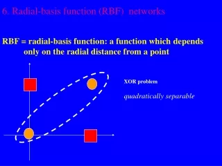
Universal Approximation Theorem • Let be a continuous function and • Let denote the family of RBF networks consisting of represented by ( ) • Universal Approximation Theorem • for any continuous function f(x), there is an RBF network with a set of centers and a common width • the realization function F(x) is close to f(x) in the Lp norm,
Curse of Dimensionality(Revisited) • The space of approximating functions attainable with MLP and RBF networks becomes increasingly constrained as the input dimensionality is increased • when the rate of convergence is , the space of approximating functions attainable : • with RBF networks : the Sobolev space, whose derivatives of the up to order are integrable • with MLP : ( : the Fourier transform of F(x)) • In other words, the curse of dimensionality can be broken neither MLP, nor RBF Networks
Relationship btw. Sample Complexity, Computational Complexity, and Generalization Performance • Two reasons of the generalization error of a neural network • approximation error : error from the limitation of the network to represent a target function • estimation error : error from the limited amount of training data • In RBF Networks with input nodes and hidden units Then the generalization error is : • where confidence parameter : , probability >= 1- • iff increases more slowly than • For a N, the optimum number of hidden units • The rate of approximation of the RBF network :
Kernel Regression(1) • Consider the nonlinear regression model : • Recall from chapter 2 : • From probability theory, • By using (2) in (1),
Kernel Regression(2) • We do not know the . So we estimate f(x) by using Parzen-Rosenblatt density estimator : • integration and by putting , and using the symmetric property of K, we get :
Kernel Regression • By using (4) and (5) as estimates of part of (3) :
Nadaraya-Watson Regression Estimator(NWRE) • By define the normalized weighting function : • We can rewrite (6) as : • F(x) : a weighted average of the y-observables
Normalized RBF Network • Assuming the spherical symmetry of K(x), then : • Then we can define the normalized radial basis function : • let for all I, we may rewrite (6) as : • may be interpreted as the probability of an event conditional on
Multivariate Gaussian Distribution(1) • If we take the kernel function as the multivariate Gaussian Distribution : • Then we can write : • So, the NWRE is :
Multivariate Gaussian Distribution(2) • And the NRBF is: • In eqs. (7) and (8), the centers of the RBF coincide with the data points