Download
1 / 47
470 likes | 569 Views
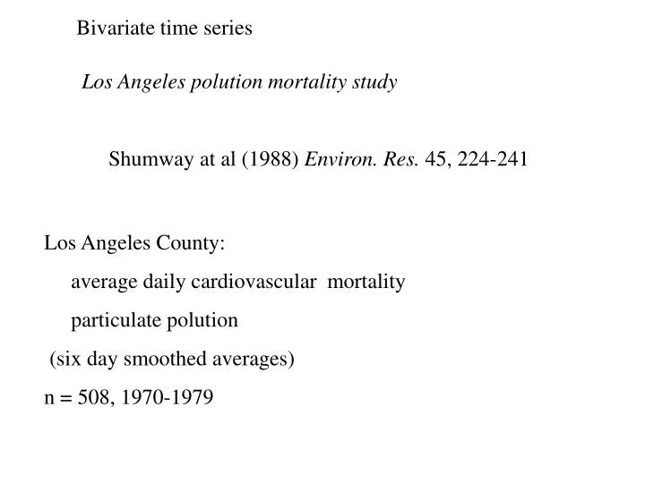
Bivariate time series. Los Angeles polution mortality study Shumway at al (1988) Environ. Res. 45, 224-241. Los Angeles County: average daily cardiovascular mortality particulate polution (six day smoothed averages) n = 508, 1970-1979. acf ccf.

E N D
Bivariate time series Los Angeles polution mortality study Shumway at al (1988) Environ. Res. 45, 224-241 Los Angeles County: average daily cardiovascular mortality particulate polution (six day smoothed averages) n = 508, 1970-1979
acf ccf Correlation is largest at 8 weeks lag, but ...
Stat 153 - 29 Oct 2008 D. R. Brillinger Chapter 9 - Linear Systems Common in nature Linear. Λ[λ1x1 + λ2x2](t) = λ1Λ[x1](t) + λ2 Λ[x2](t) Time invariant. Λ[Bτx](t) = BτΛ[x](t) Λ[Bτx](t) = y(t- τ) if Λ[x](t) = y(t) Example. How to describe ?
System identification Yt = hk Xt-k + Nt Is there a relationship? Estimate h, H given {x(t),y(t)}, t=0,...,N Predict Y from X Control Studying causality Studying delay …
One way {hk}: impulse response Define δk= 1 if k = 0 and = 0 otherwise, then hk = 0 k<0: causal/physically realizable
Transfer / frequency response function Another way complex-valued G(ω ) = |H(ω)|:gain φ(ω) = arg{H(ω)}: phase H(ω+2π) = H(ω) H(-ω) = H(ω)* complex conjugate
Example. H(ω) = (1+2cos ω)/3
Fundamental property of a linear time invariant system If input x(t) = exp{-iωt}, then output y(t) = H(ω)exp{-iωt} cosinusoids are carried into cosinusoids of the same frequency frequencies are not mixed up If (useful approximation) then
Ideal low-pass filter H(ω ) = 1 |ω| Ω = 0 otherwise, |ω| π
Ideal band-pass filter H(ω ) = 1 |ω-ω0| Δ = 0 otherwise
Construction of general filter via fft( ) Inverse Filtered series
Bandpass filtering of Vienna monthly temperatures, 1775-1950 Bank of bandpass filters Taper, form g(t/(N+1)xt, t=1,...,N e.g. g(u) = (1 + cos πu)/2
Pure lag filter. y = xt-τ hk = 1 if k = τ = 0 otherwise H(ω ) = exp{-iωτ} φ(ω) = -ωτ mod(2π) G(ω) = 1
Product sales and a leading indicator series Box and Jenkins
acf ccf
Work with differences -prewhitening
The effect of filtering on second-order parameters γYY (k) = Σ Σ hi hj γXX (k-j+i) Proof. Cov{yt+k ,xt } =
fYY(ω) = |H(ω)|2 fXX(ω) Proof. fYY (ω)= Σ γYY(k) exp{-iωk}]/π = ΣΣ Σ hi hj γXX (k-j+i) exp{-iωk}]/π
Interpretation of fXX(ω0) γYY (0) = var Yt = fYY(ω)dω = |H(ω)|2 fXX(ω)dω f(ω0) if H(.) narrow bandpass centered at ω0 Provides an estimate of f(ω0) ave{xt (ω0)2}
Remember The narrower the filter the less biased the estimate, generally.
The coherence may be estimated via estimate of corr{xt (ω),yt(ω)}2 and … Hilbert transform
Another estimate fYY(ω) = |H(ω)|2 fXX(ω) suggests e.g. fit AR(p), p large
Spectral density of an AR(p) Proof fYY(ω) = |H(ω)|2 fXX(ω) φ(B)Yt = Zt
Spectral density of an ARMA(p,q) Proof. fYY(ω) = |H(ω)|2 fXX(ω) φ(B)Yt = θ(B)Zt
System identification Yt = hk Xt-k + Nt Black box What is inside?
Estimating the frequency response function Yt = hk Xt-k + Nt Yt = h(B) Xt + Nt γXY (τ) = Σ hk γXX (τ-k) fXY(ω) = H(ω)fXX(ω) Proof
Estimate Form estimates by smoothing m periodograms Coherence/squared coherency Expected value m/M in case C(ω)=0 Upper 100α% null point 1-(1-α)1/(m-1)
Took m = 5 Lag of about 3 days
Gas furnace data Cross-spectral analysis nonparametric model Input: (.6 - methane feed)/.04 Output: percent CO2 in outlet gas
acf ccf
Box-Jenkins approach Yt = h(B) Xt-k + Nt h(B) = δ(B)-1ω(B)Bb Parametric model E.g. furnace data Yt = ω0Xt+...+ω11Xt-11+β0Zt+...+β9Zt-9 impulse response {ωk}
Discussion Plot the data (xt , yt ), t=1,...,N time side vs. frequency side quantities acf, ccf fYY , fXY, C {hk} H(ω) parametric vs. nonparametric models ARMAX(p,q) Yt = hk Xt-k + Nt
MA(q): Yt = Xt + β1 Xt-1 + ... + βq Xt-q AR(p): Yt = α1Yt-1 + α2Yt-2 + ... + αpYt-p + Xt ARMA(p,q): Yt = α1Yt-1 + α2Yt-2 + ... + αpYt-p + Xt + β1 Xt-1 + ... + βq Xt-q φ(B)Yt = θ(B)Xt Yt = φ(B)-1θ(B)Xt
Yt = φ(B)-1θ(B)Xt MA(q): Yt = Xt + β1 Xt-1 + ... + βq Xt-q AR(p): Yt = α1Yt-1 + α2Yt-2 + ... + αpYt-p + Xt ARMA(p,q): Yt = α1Yt-1 + α2Yt-2 + ... + αpYt-p + Xt + β1 Xt-1 + ... + βq Xt-q
ARMA(p,q): Yt = α1Yt-1 + α2Yt-2 + ... + αpYt-p + Xt + β1 Xt-1 + ... + βq Xt-q Yt = φ(B)-1θ(B)Xt