Download
1 / 54
540 likes | 556 Views
An apprenticeship learning algorithm that produces simpler apprentice policies, faster than previous methods, aiming to match or improve expert policies based on demonstrations. The approach involves linear programming and basis reward functions. The algorithm outputs a single stationary policy for efficient learning. The linear program is designed to find the apprentice policy that maximizes value based on the expert's demonstrations. It simplifies the learning process and is empirically faster, making it advantageous over traditional methods.

E N D
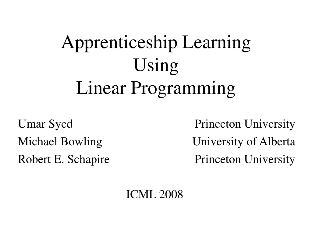
Apprenticeship Learning: An apprentice learns to behave by observing an expert. Learning algorithm Output: Apprentice policy that is at least as good as expert policy (and possibly better). Input: Demonstrations by expert policy.
Main Contribution A new apprenticeship learning algorithm that: Produces simpler apprentice policies, and Is empirically faster than previous algorithms.
Outline Introduction Apprenticeship Learning Prior Work Summary of Advantages Over Prior Work Background: Occupancy Measure Linear Program for Apprenticeship Learning (LPAL) Experiments and Demos Other Topics
Given:Same as Markov Decision Process, except no reward function R. Also given: Basis reward functions R1, …, Rk. Demonstrations by an expert policy ¼E. Assume: True reward function R is a weighted combination of the k basis reward functions: R(s, a) = iwi* ¢ Ri(s, a) where weight vector w* is unknown. Goal: Find apprentice policy ¼A such that V(¼A) ¸ V(¼E) where value V(¼) of policy ¼ is with respect to unknown reward function. Apprenticeship Learning
Outline Introduction Apprenticeship Learning Prior Work Summary of Advantages Over Prior Work Background: Occupancy Measure Linear Program for Apprenticeship Learning (LPAL) Experiments and Demos Other Topics
Define Vi(¼) = ith “basis value” of ¼ = Value of ¼ with respect to ith basis reward function. Then true value of a policy is a weighted combination of its basis values, i.e. V(¼) = iwi*¢Vi(¼) Proof: Linearity of expectation. Prior Work – Key Idea
Introduced the apprenticeship learning framework. Algorithm Idea: Estimate Vi(¼E) for all i from expert’s demonstrations. Find ¼A such that Vi(¼A) = Vi(¼E) for all i. Theorem: V(¼A) = V(¼E) Algorithm “type”:Geometric Prior Work – Abbeel & Ng (2004)
Assumed that all wi* are non-negative and sum to 1. Algorithm Idea: Estimate Vi(¼E) for all i from expert’s demonstrations. Find ¼A and M such that: Vi(¼A) ¸Vi(¼E) + M for all i, and M is as large as possible. Theorem: V(¼A) ¸ V(¼E), and possibly V(¼A) À V(¼E). Algorithm “type”:Boosting Prior Work – Syed & Schapire (2007)
Outline Introduction Apprenticeship Learning Prior Work Summary of Our Approach Background: Occupancy Measure Linear Program for Apprenticeship Learning (LPAL) Experiments and Demos Other Topics
Same algorithm idea as Syed & Schapire (2007), but formulated as a single linear program, which we give to an off-the-shelf solver. Summary of Our Approach
Previous algorithms: Didn’t actually output a single stationary policy ¼A, but instead output a distributionD over a set of stationary policies, such that E¼ »D[V(¼A)] ¸ V(¼E) Our algorithm: Outputs a single stationary policy ¼A such that V(¼A) ¸ V(¼E), and possibly V(¼A) À V(¼E). Advantage: Apprentice policy is simpler and more intuitive. Advantages of Our Approach A
Advantages of Our Approach • Previous algorithms: Ran for several rounds, and each round required solving a standard MDP (expensive). • Our algorithm: A single linear program. • Advantage: Empirically faster than previous algorithms. • We informally conjecture that this is because it solves the problem “all at once”.
Outline Introduction Apprenticeship Learning Prior Work Summary of Our Approach Background: Occupancy Measure Linear Program for Apprenticeship Learning (LPAL) Experiments and Demos Other Topics
The occupancy measurex¼2R|S||A| of policy ¼is an alternate way of describing how ¼ moves through the state-action space. x¼sa = Expected (discounted) number of visits by policy ¼ to state-action pair (s, a). Example: Suppose policy ¼ visits state-action pair (s, a): With probability 1 at time 1. With probability 1/2 at time 2. With probability 1/3 at time 3. With probability 0 a time ¸ 4. Then x¼sa = 1 + °(1/2) + °2(1/3) Occupancy Measure
Occupancy Measure – Equivalent Representation The relationship between a stationary policy ¼and its occupancy measure x¼is given by: Proof: Left-hand side = Probability of taking action a in state s. Right-hand side = No. of visits to state-action (s, a) No. of visits to state s. Significance: It is easy to recover a stationary policy from its occupancy measure.
Define º(x) ,s,a R(s, a) ¢xsa Then V(¼) = º(x¼). In other words, º(x) is the value of a policy whose occupancy measure is x. Proof: A policy earns reward R(s, a) (suitably discounted) every time it visits state-action pair (s, a). Significance: The value of a policy is a linear function of its occupancy measure. Occupancy Measure – Calculating Value
Occupancy Measure – Bellman Flow Constraints The Bellman flow constraints are a set of constraints that any vector x2R|S||A| must satisfy to be a valid occupancy measure. The Bellman flow constraints say: “Under any policy, the number of visits into a state s must equal the number of visits leaving state s.” s Must be equal
Occupancy Measure – Bellman Flow Constraints In fact, the Bellman flow constraints completely characterize the set of occupancy measures. x satisfies the Bellman flow constraints m x is the occupancy measure of some policy ¼ Significance: The Bellman flow constraints are linear in x. All policies All occupancy measures ¢¼ x ¢ Bellman flow constraints
Outline Introduction Apprenticeship Learning Prior Work Summary of Our Approach Background: Occupancy Measure Linear Program for Apprenticeship Learning (LPAL) Experiments and Demos Other Topics
Derivation of LPAL Algorithm 1. Estimate Vi(¼E) for all i from expert’s demonstrations. 2. Find ¼A and M that solve: max M subject to: Vi(¼A) - Vi(¼E) ¸ M for all i. ¼A is a policy. Start with algorithm idea from Syed & Schapire (2007)
Derivation of LPAL Algorithm 1. Estimate Vi(¼E) for all i from expert’s demonstrations. 2. Find ¼A and M that solve: max M subject to: Vi(¼A) - Vi(¼E) ¸ M for all i. ¼A is a policy. xA satisfies the Bellman flow constraints. xA
Derivation of LPAL Algorithm 1. Estimate Vi(¼E) for all i from expert’s demonstrations. 2. Find ¼A and M that solve: max M subject to: Vi(¼A) - Vi(¼E) ¸ M for all i. ¼A is a policy. xA satisfies the Bellman flow constraints. xA ºi(xA)
Derivation of LPAL Algorithm 1. Estimate Vi(¼E) for all i from expert’s demonstrations. 2. Find¼Aand M that solve: max M subject to: Vi(¼A) - Vi(¼E) ¸ M for all i. ¼A is a policy xA satisfies the Bellman flow constraints. xA ¼A ºi(xA) Vi(¼A) ¼A is a policy.
Derivation of LPAL Algorithm 1. Estimate Vi(¼E) for all i from expert’s demonstrations. 2. Find xA and M that solve: max M subject to: ºi(xA) - Vi(¼E) ¸ M for all i. xA satisfies the Bellman flow constraints.
Derivation of LPAL Algorithm 1. Estimate Vi(¼E) for all i from expert’s demonstrations. 2. Find xA and M that solve: max M subject to: ºi(xA) - Vi(¼E) ¸ M for all i. xA satisfies the Bellman flow constraints. This is a linear program!
Derivation of LPAL Algorithm 1. Estimate Vi(¼E) for all i from expert’s demonstrations. 2. Find xA and M that solve: max M subject to: ºi(xA) - Vi(¼E) ¸ M for all i. xA satisfies the Bellman flow constraints. “Of all occupancy measures …
Derivation of LPAL Algorithm 1. Estimate Vi(¼E) for all i from expert’s demonstrations. 2. Find xA and M that solve: max M subject to: ºi(xA) - Vi(¼E) ¸ M for all i. xA satisfies the Bellman flow constraints. “Of all occupancy measures … find one corresponding to a policy that is better than the expert’s policy …
Derivation of LPAL Algorithm 1. Estimate Vi(¼E) for all i from expert’s demonstrations. 2. Find xA and M that solve: max M subject to: ºi(xA) - Vi(¼E) ¸ M for all i. xA satisfies the Bellman flow constraints. “Of all occupancy measures … find one corresponding to a policy that is better than the expert’s policy … by as much as possible.”
Derivation of LPAL Algorithm 1. Estimate Vi(¼E) for all i from expert’s demonstrations. 2. Find xA and M that solve: max M subject to: ºi(xA) - Vi(¼E) ¸ M for all i xA satisfies the Bellman flow constraints. “Of all occupancy measures … find one corresponding to a policy that is better than the expert’s policy … by as much as possible.” 3. Convert occupancy measure to a stationary policy:
Theorem: V(¼A) ¸ V(¼E), and possibly V(¼A) À V(¼E). (same as Syed & Schapire (2007)) Proof: Almost immediate. Remark: We could have applied the same occupancy measure “trick” to the algorithm idea from Abbeel & Ng (2004), and likewise derived a linear program. LPAL Algorithm
Outline Introduction Apprenticeship Learning Prior Work Summary of Our Approach Background: Occupancy Measure Linear Program for Apprenticeship Learning (LPAL) Experiments and Demos Other Topics
Experiment – Setup • Actions & transitions: North, South, East and West, with 30% chance of moving to a random state. • Basis rewards: One indicator basis reward per region. • Expert: Optimal policy for randomly chosen weight vector w*. “Gridworld” environment, divided into regions Region State
Experiment – Setup • Compare: • Projection algorithm (Abbeel & Ng 2004) • MWAL algorithm (Syed & Schapire 2007) • LPAL algorithm (this work) • Evaluation Metric: Time required to learn apprentice policy whose value is 95% of the optimal value.
Experiment – Results Note: Y-axis is log scale.
Experiment – Results Note: Y-axis is log scale.
Demo – Mimicking the Expert Output of LPAL algorithm Expert
Demo – Improving Upon the Expert Output of LPAL algorithm Expert
Outline Introduction Apprenticeship Learning Prior Work Summary of Our Approach Background: Occupancy Measure Linear Program for Apprenticeship Learning (LPAL) Experiments and Demos Other Topics
Also Discussed in the Paper… • We observe that the MWAL algorithm often performs better than its theory predicts it should. • We have new results explaining this behavior (in preparation).
Constrained MDPs and RL with multiple rewards: Feinberg and Schwartz (1996) Gabor, Kalmar and Szepesvari (1998) Altman (1999) Shelton (2000) Dolgov and Durfree (2005) … Max margin planning: Ratliff, Bagnell and Zinkevich (2006) Related to Our Approach
Recap A new apprenticeship learning algorithm that: Produces simpler apprentice policies, and Is empirically faster than previous algorithms. Thanks! Questions?
Algorithms for finding ¼A: Max-Margin: Based on quadratic programming. Projection: Based on a geometric approach. MWAL: Based on a multiplicative weights approach, similar to boosting. Actually, existing algorithms don’t find a single stationary ¼A, but instead find a distributionD over a set of stationary policies, such that E¼»D[V(¼A)] ¸ V(¼E). Drawbacks: Apprentice policy is nonintuitive and complicated to describe. Algorithms have slow empirical running time. Prior Work – Details
Same algorithm idea: Find ¼A such that Vi(¼A) ¸Vi(¼E) for all i. Algorithm to find ¼A based on linear programming. Allows us to leverage the efficiency of modern LP solvers. Outputs a single stationary policy ¼A such that V(¼A) ¸ V(¼E). Benefits: Apprentice policy is simpler. Algorithm is empirically much faster. This Work
Same algorithm idea: Find ¼A such that Vi(¼A) ¸Vi(¼E) for all i. Algorithm to find ¼A based on linear programming. Allows us to leverage the efficiency of modern LP solvers. Outputs a single stationary policy ¼A such that V(¼A) ¸ V(¼E). Benefits: Apprentice policy is simpler. Algorithm is empirically much faster. This Work
The occupancy measurex¼2R|S||A| of policy ¼is an alternate way of describing how ¼ moves through the state-action space. x¼sa = Expected (discounted) number of visits by policy ¼ to state-action pair (s, a). Occupancy Measure – Equivalent Representation
Given the occupancy measure x¼of a policy ¼, computing the basis values of ¼is easy. Define ºi(x) ,s,a Ri(s, a) ¢xsa Then V_i(\pi) = \nu_i(x^\pi). In other words, \nu_i(x) is the ith basis value of a policy whose occupancy measure is x. Proof: Policy ¼ earns (suitably discounted) reward Ri(s, a) for each visit to state-action pair (s, a). And x¼sa is the expected (and suitably discounted) number of visits by policy ¼ to state-action pair (s, a). Occupancy Measure – Calculating Value
Occupancy Measure – Calculating Value Given the occupancy measure x¼of a policy ¼, computing the basis values of ¼is easy: Vi(¼) = s,a Ri(s, a) ¢x¼(s, a) Proof: Linearity of expectation. For convenience, define: ºi(x) , s,a Ri(s, a) ¢x(s, a)
Define º(x) ,s,a R(s, a) ¢xsa Then V(¼) = º(x¼). In other words, º(x) is the value of a policy whose occupancy measure is x. Proof: Policy ¼ earns (discounted) reward R(s, a) for each visit to state-action pair (s, a). And x¼sa is the expected (discounted) number of visits by policy ¼ to state-action pair (s, a). So V(\pi) is Occupancy Measure – Calculating Value
Occupancy Measure – Bellman Flow Constraints The Bellman flow constraints are a set of linear constraints that define the set of all occupancy measures. x satisfies the Bellman flow constraints m x is the occupancy measure of some policy ¼ All policies All occupancy measures ¢¼ x ¢ Bellman flow constraints