Download
1 / 58
580 likes | 662 Views
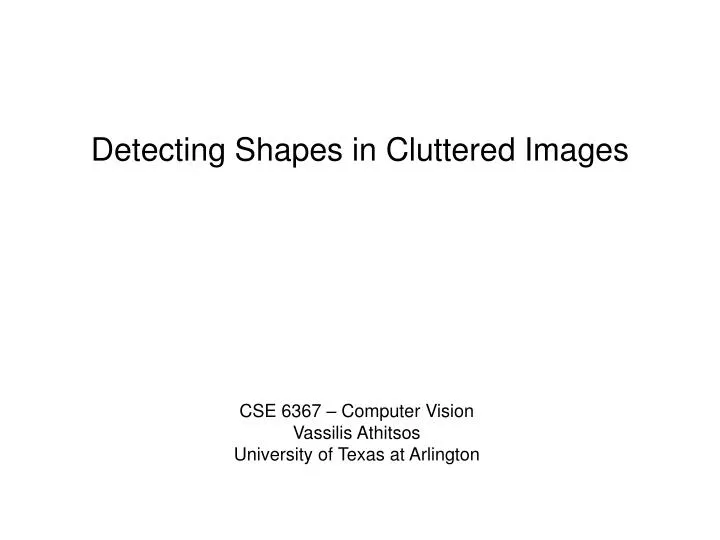
Detecting Shapes in Cluttered Images. CSE 6367 – Computer Vision Vassilis Athitsos University of Texas at Arlington. Objects with parts that can: Occur an unknown number of times. Leaves, comb teeth. Be not present at all. Leaves, comb teeth, fingers. Have alternative appearances.

E N D
Detecting Shapes in Cluttered Images CSE 6367 – Computer Vision Vassilis Athitsos University of Texas at Arlington
Objects with parts that can: Occur an unknown number of times. Leaves, comb teeth. Be not present at all. Leaves, comb teeth, fingers. Have alternative appearances. Fingers. Objects With Variable Shape Structure branches combs hands
Other Examples • Satellite Imaging parking lot residential neighborhood boat pier
Roadways highway exits
Other Examples • Medical Imaging ribs & bronchial tree
Goal: Detection in Cluttered Images Branches Hands
Deformable Models Not Adequate • Shape Modeling: • “Shape deformation” ≠ “structure variation” ∩
Limitations of Fixed-Structure Methods • A different model is needed for each fixed structure.
Limitations of Fixed-Structure Methods • Worst case: number of models is exponential to number of object parts.
Overview of Approach • Hidden Markov Models (HMMs) can generate shapes of variable structure. • HMMs cannot be matched to an image. • Image features are not ordered. • Many (possibly most) features are clutter. • Solution: Hidden State Shape Models.
An HMM for Branches of Leaves end state • Each box is a state. • Arrows show legal state transitions. top leaf initial state stem right leaf left leaf
An HMM for Branches of Leaves end state stem • Each box is a state. • For each state there is a probability distribution of shape appearance. top leaf initial state stem right leaf left leaf left leaf
Generating a Branch end state • Choose a legal initial state. • Choose a shape from the state’s shape distribution. top leaf initial state stem right leaf left leaf
Generating a Branch end state • Choose a legal initial state. • Choose a shape from the state’s shape distribution. top leaf initial state stem right leaf left leaf
Generating a Branch end state • Choose a legal initial state. • Choose a shape from the state’s shape distribution. top leaf initial state stem right leaf left leaf
Generating a Branch end state • Choose a legal transition to a next state. • Choose a shape from the next state’s shape distribution. top leaf initial state stem right leaf left leaf
Generating a Branch end state • Choose a legal transition to a next state. • Choose a shape from the next state’s shape distribution. top leaf initial state stem right leaf left leaf 17
Generating a Branch end state • Choose a legal transition to a next state. • Choose a shape from the next state’s shape distribution. top leaf initial state stem right leaf left leaf
Generating a Branch end state • Choose a legal transition to a next state. • Choose a shape from the next state’s shape distribution. top leaf initial state stem right leaf left leaf
Generating a Branch end state • Choose a legal transition to a next state. • Choose a shape from the next state’s shape distribution. top leaf initial state stem right leaf left leaf
Generating a Branch end state • Choose a legal transition to a next state. • Choose a shape from the next state’s shape distribution. top leaf initial state stem right leaf left leaf
Generating a Branch end state • Choose a legal transition to a next state. • Choose a shape from the next state’s shape distribution. top leaf initial state stem right leaf left leaf
Generating a Branch end state • Can stop when at a legalend state. top leaf initial state stem right leaf left leaf
An HMM for Handshapes • Each circle is a state (object part). • Arrows show legal state transitions.
Matching Observations via DTW end state • Given a sequence of shape parts, what is the optimal sequence of corresponding states? top leaf initial state stem right leaf left leaf
Matching Observations via DTW 9 end state • Given a sequence of shape parts, what is the optimal sequence of corresponding states? top leaf 8 7 6 5 initial state stem right leaf 4 3 left leaf 2 1
Matching Observations via DTW end state 9 top leaf • The Viterbi algorithm produces aglobally optimal answer. top leaf 7 left leaf 8 stem 6 stem initial state 5 rightleaf stem right leaf 4 stem 3 leftleaf left leaf 2 stem 1 stem
DTW/HMMs Cannot Handle Clutter 9 8 7 6 5 4 3 2 1 clean image, ordered observations DTW/HMM can parse theobservations cluttered image, unordered observations
Key Challenges in Clutter • The observations are not ordered. • Many (possibly most) observations should not be matched. • Solution: Hidden State Shape Models (HSSMs). • Extending HMMs and the Viterbi algorithm to address clutter.
Inputs end state • Shape Model. • Shape parts. • Legal transitions. • Initial/end states. • More… top leaf possible leaf locations initial state stem right leaf left leaf possible stem locations • Possible matches for each model state.
possible stem locations Algorithm Input/Ouptut • Input: Set of K image features {F1, F2, …, FK}. possible leaf locations oriented edge pixels
Algorithm Input/Output • Input: Set of K image features {F1, F2, …, FK}. • Output: Registration. • ((Q1, O1), (Q2, O2), …, (QT, OT)). • Sequence of matches. Qj: model state. : Oj feature. • Model states tell us the structure. • Features tell us the location.
Algorithm Input/Output • Input: Set of K image features {F1, F2, …, FK}. Q1: stem • Output: Registration. • ((Q1, O1), (Q2, O2), …, (QT, OT)). • Sequence of matches. Qj: model state. : Oj feature. • Model states tell us the structure. • Features tell us the location.
Algorithm Input/Output • Input: Set of K image features {F1, F2, …, FK}. Q2: left leaf • Output: Registration. • ((Q1, O1), (Q2, O2), …, (QT, OT)). • Sequence of matches. Qj: model state. : Oj feature. • Model states tell us the structure. • Features tell us the location.
Algorithm Input/Output • Input: Set of K image features {F1, F2, …, FK}. Q3: stem • Output: Registration. • ((Q1, O1), (Q2, O2), …, (QT, OT)). • Sequence of matches. Qj: model state. : Oj feature. • Model states tell us the structure. • Features tell us the location.
Algorithm Input/Output • Input: Set of K image features {F1, F2, …, FK}. Q4: right leaf • Output: Registration. • ((Q1, O1), (Q2, O2), …, (QT, OT)). • Sequence of matches. Qj: model state. : Oj feature. • Model states tell us the structure. • Features tell us the location.
Algorithm Input/Output • Input: Set of K image features {F1, F2, …, FK}. top leaf left leaves right leaves stem • Output: Registration. • ((Q1, O1), (Q2, O2), …, (QT, OT)). • Sequence of matches. Qj: model state. : Oj feature. • Model states tell us the structure. • Features tell us the location.
Finding the Optimal Registration top leaf left leaves right leaves stem optimal registration some possible registrations • Number of possible registrations is exponential to number of image features. • Evaluating each possible registration is intractable. • We can find optimal registration in polynomial time (quadratic/linear to the number of features). • Using dynamic programming (modified Viterbi).
Evaluating a Registration • Registration: • ((Q1, O1), (Q2, O2), (Q3, O3), (Q4, O4), …, (QT, OT)). • Probability is product of: • I(Q1): prob. of initial state. • B(Qj, Oj): prob. of feature given model state. • A(Qj, Qj+1): prob. of transitionfrom Qj to Qj+1. • D(Qj, Oj, Qj+1, Oj+1): prob. ofobserving Oj+1 given state = Qj+1, and given previous pair (Qj, Oj). • Not in HMMs, because therethe order is known. top leaf left leaves right leaves stem optimal registration
Finding the Optimal Registration • Dynamic Programming algorithm: • Break up problem into smaller, interdependent problems. • Definition: W(i, j, k) is the optimal registration such that: • Registration length is j. • Qj = Si. • Oj = Fk. • Optimal registration: • W(i, j, k) with highest probability, such thatQj is a legal end state. • Suffices to compute all W(i, j, k). O4 Q4: right leaf
Finding the Optimal Registration • W(i, j, k): highest prob. registration such that: • Registration length is j. • Qj = Si. • Oj = Fk. • W(i, 1, k) is trivial: only one choice. • Registration consists of pairing Si with Fk. • Cost: I(Si) + B(Si, Fk): • W(i, 2, k) is non-trivial: we have choices. • Registration: ((Q1, O1), (Q2, O2)) • Q2 = Si, O2 = Fk. • What we do not know: Q1, O1. • We can try all possible (Q1, O1), not too many.
Finding the Optimal Registration • W(i, 3, k): even more choices. • Registration: ((Q1, O1) , (Q2, O2), (Q3, O3)) • Q3 = Si, O3 = Fk. • What we do not know: Q1, O1, Q2, O2. • Here we use dynamic programming. • W(i, 3, k) = ((Q1, O1) , (Q2, O2), (Q3, O3)) implies thatW(i’, 2, k’) = ((Q1, O1) , (Q2, O2)). • If we have computed all W(i, 2, k), the number of choices for W(i, 3, k) is manageable. • This way we compute W(i, j, k) for all j. • The number of choices does no increase with j.
Unknown-scale Problem What is the length of the optimal registration? T = 800 T = 400 T = 600 T= 1000 T = 500 T = 800 • Probability decreases with registration length. • HMMs are biased towards short registrations
Unknown-scale Problem What is the length of the optimal registration? C B A • Probability decreases with registration length. • HMMs are biased towards short registrations
Handling Unknown Scale • Registration: • ((Q1, O1), (Q2, O2), (Q3, O3), (Q4, O4), …, (QT, OT)). • Probability is product of: • I(Q1): prob. of initial state. • B(Qj, Oj): prob. of feature given model state. • A(Qj, Qj+1): prob. of transitionfrom Qj to Qj+1. • D(Qj, Oj, Qj+1, Oj+1): prob. ofobserving Oj+1 given state = Qj+1, and given previous pair (Qj, Oj).
Handling Unknown Scale • Registration: • ((Q1, O1), (Q2, O2), (Q3, O3), (Q4, O4), …, (QT, OT)). • Probability is product of: • I(Q1): prob. of initial state. • B(Qj, Oj): prob. of feature given model state. • A(Qj, Qj+1): prob. of transitionfrom Qj to Qj+1. • D(Qj, Oj, Qj+1, Oj+1): prob. ofobserving Oj+1 given state = Qj+1, and given previous pair (Qj, Oj).
P(Oj | Qj) P(Oj | clutter) Handling Unknown Scale • Before: B(Qj, Oj): prob. of feature given state. • Adding a feature decreases registration probability. • Now: B(Qj, Oj) is a ratio: • B(Qj, Oj) can be greater or less than 1. • Adding a feature may increase or decrease registration probability. • Bias towards short registrations is removed.
Another Perspective • Before: probability depended only on features matched with the model. • Fewer features higher probability. • The probability function shouldconsider the entire image. • Features matched with model. • Features assigned to clutter.
Another Perspective • For every feature, does it match better with the model or with clutter? • Compute P(Fk | clutter). • Given a registration R, define: • C(R): set of features left out. • F: set of all image features. • Total probability: • P(registration) P(C(R) | clutter)). C(R): gray F: gray/black
P(registration) P(C(R) | clutter)) P(F | clutter)) Another Perspective • Given a registration R, define: • C(R): set of features left out. • F: set of all image features. • Total probability: • P(registration) P(C(R) | clutter)) proportional to: C(R): gray F: gray/black