Download
1 / 70
730 likes | 1.01k Views
Optimal Groundwater Remediation. Laura Place Taren Blue. Outline. Background What is Groundwater Remediation Major Contaminants and Contamination Areas The Remediation Process Treatment Methods Mathematical Models Optimization Completed Work Fluid Flow Modeling

E N D
Optimal Groundwater Remediation Laura Place Taren Blue
Outline • Background • What is Groundwater Remediation • Major Contaminants and Contamination Areas • The Remediation Process • Treatment Methods • Mathematical Models • Optimization • Completed Work • Fluid Flow Modeling • Plans and Recommendations for Future Work
Background • Groundwater Remediation • Removal of contaminants from a water supply • Standards set by the EPA • Several methods for treatment • Existing • Experimental • Optimization • Mathematical models
Background • Sources of contamination • Industrial & agricultural • Storage tanks • Septic systems • Landfills • Hazardous waste sites • Road salts • Refinery operations • Mining • Other chemicals
Where are the Problem Areas? Nitrates Arsenic Hard Water VOCs
Optimization • Goals • Minimize the remaining contaminants • Minimize cost • Costs minimized are unique to the model • Other goals are also unique to the specific model • Optimizing the pump treat inject method (PTI) • Number of wells • Well configuration
What are the Choices? • “Dilution is not the solution!!!” • Inexpensive but never resolves the problem • Pump, Treat, Inject method (PTI) • Pump contaminated water from the source (the plume) • Treat the water • Inject treated water back into the aquifer
Treatments • Existing treatment methods • Ion exchange chromatography • Membranes • “Point of service” treatment • Bioreactors • Adsorption • In situ bioremediation • Liquid-liquid extraction • Surfactants
Challenges of Remediation • Plume • Unknown flow patterns • Unknown concentration profiles • Nonuniformities in concentration • Unknown position • Uncertainty in composition • Unknown size • Geological uncertainty
Problems and Affect on Treatment ***Modeling of the aquifer depends on many of these parameters. Therefore, all of these issues also become a problem in mathematical modeling.
PTI • Has many parameters • Number and location of wells • Few large wells • Many small wells • Pumping Rate • Concentration of contaminants in treated water • Can vary well arrangement with time • For optimization – Need a model!
Well Position and Treatment Four different well arrangements. ***Concentration profile of the plume is affected by location of pumping and injection wells.
Steps Completed in Optimization • Analytical Model • Euler Approximation • Optimization for minimum cost • Initial Fluid Flow Modeling and Analysis • Refined Fluid Flow Modeling and Analysis • Optimization for minimum contamination
Set Up Euler Approximation • Where • dc/dt is the change in concentration with time • Fp is the pumping rate • cin is the concentration into the slice • cout is the concentration out of the slice • Vslice is the volume of the slice
Euler Method Model • Calculates total remediation time • Uses inputs for: • Volume of the plume • Time steps • Flow rate • Initial concentration • Desired end concentration • Calculation in each cell loops until the change in outlet concentration is < 0.0001
Euler Results t1 t2
Fluid Flow Analysis Arrangement Example of one arrangement – multiple outlets with one inlet
Fluent • Calculate mass flow rates in the plume • More accurate approximations of concentration profiles • Characterize fluid flow in the aquifer • Vary well arrangement • Vary number of injection and extraction sites • Vary pumping rate
Geometry - Gambit • 1st “draw” geometry in Gambit • Create injection and extraction locations which may be turned on or off. • For off – face is treated as a wall • For on – face is designated either mass inlet or outflow • Each face is labeled by location
Generic Geometry 10 20 10 A B C D E F G 1 2 3 4 5 6 7
Define Geometry in Fluent One outlet One inlet
Imaginary Planes A B C • Fluent analyzes flow patterns through planes I J K D L M N E O P Q F G H
Example of Fluid Flow Field in Fluent Flow rate of 50 kg/s
Example of Fluid Flow Field in Fluent Flow rate of 5 kg/s
Example of Velocity Contours Flow rate of 5 kg/s
Excel • Results from Fluent imported into Excel
Mass Balance C-18 C-14 C-10 Negative flux or positive flux dictates which concentration to use in the mass balance
Remediation Time and Flow Rate (2,1) (1,1) (4,1) (1,4) (4,4) (2,2) (1,2)
Conclusions of this Model • Imaginary planes give an accurate estimate of flow through the aquifer • Flux through the planes can be used to describe concentration profiles with time • This model allows for understanding of general flow patterns with configuration • Gives basis of comparison for future modeling techniques
New Modeling Strategy • Pipes in the top of the aquifer • More realistic injection modeling • Flow characteristics re-evaluated • Several plume types evaluated • Non-uniform initial concentrations • Different shapes • Injection and extraction varied with time • More realistic aquifer shape
Naming the Wells 1 2 3 4 5 6 7 A B C D
Planes Through the x-direction -18 -14 -10 … 18
Horizontal Planes Horizontal planes also named individually for x, y and z location in the aquifer.
Model Aquifer with Non-Uniform Concentration • 3 plumes analyzed
Schemes for TreatmentPlume 1 Step 1 Step 2 Step 3
Schemes for TreatmentPlume 2 Step 1 Step 2 Step 3
Schemes for TreatmentPlume 3 Step 1 Step 2 Step 3