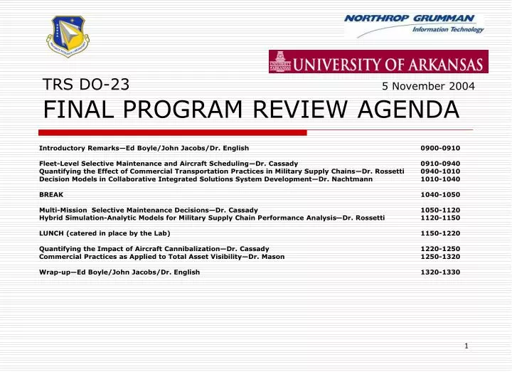
TRS DO-23 5 November 2004 FINAL PROGRAM REVIEW AGENDA

1. TRS DO-23 5 November 2004FINAL PROGRAM REVIEW AGENDA Introductory Remarks—Ed Boyle/John Jacobs/Dr. English 0900-0910 Fleet-Level Selective Maintenance and Aircraft Scheduling—Dr. Cassady 0910-0940 Quantifying the Effect of Commercial Transportation Practices in Military Supply Chains—Dr. Rossetti 0940-1010 Decision Models in Collaborative Integrated Solutions System Development—Dr. Nachtmann 1010-1040 BREAK 1040-1050 Multi-Mission Selective Maintenance Decisions—Dr. Cassady 1050-1120 Hybrid Simulation-Analytic Models for Military Supply Chain Performance Analysis—Dr. Rossetti 1120-1150 LUNCH (catered in place by the Lab) 1150-1220 Quantifying the Impact of Aircraft Cannibalization—Dr. Cassady 1220-1250 Commercial Practices as Applied to Total Asset Visibility—Dr. Mason 1250-1320 Wrap-up—Ed Boyle/John Jacobs/Dr. English 1320-1330

2. Center for Engineering Logistics and Distribution (CELDi) A National Science Foundation sponsored Industry/University Cooperative Research Center (I/UCRC)

3. Mission CELDi • CELDi provides creative, leading edge solutions to real-world problems • Sponsors collaborate with research teams • Benefit from shared research solutions • Employment of a systems perspective and an engineering approach • TheCenter for Engineering Logistics and Distribution (CELDi)is a multi-university, multi-disciplinary National Science Foundation sponsored Industry/University Cooperative Research Center (I/UCRC). Research endeavors are driven and sponsored by representatives from a broad range of member organizations, including manufacturing, maintenance, distribution, transportation, information technology, and consulting. CELDi emerged in 2001 from The Logistics Institute (1994) to provide integrated solutions to logistics problems, through research related to modeling, analysis and intelligent-systems technologies. • Research Program • The Center helps industry partners excel by leveraging their supply chain to achieve a distinguishable, sustainable difference. Through basic research, collaborative applied research with industry, technology transfer, and education, the Center is a catalyst for developing the engineering logistics methodology necessary for logistics value chain optimization. • Value-adding processes that create time and place utility (transportation, material handling, and distribution) • Value-sustaining processes that prolong useful life (maintenance, repair, and rework) • Value-recovering processes that conserve scarce resources and enhance societal goodwill (returns, refurbishment, and recycling)

4. DoD Related Logistics Partners • Defense Logistics Agency • Naval Supply Command Systems • Pine Bluff Arsenal • Raytheon Systems Company • Red River Army Depot

5. Federal Appropriation: Background • Based on research experience and collaboration with current/past I/UCRC members • Pursued multi-year appropriation to support military logistics research • History: • Congressional office visits • Beginning in mid-90’s • UA representatives • Chancellor, Provost, John English, Rick Malstrom, Van Scoyoc Associates, Inc. • Resulting in sufficient support for appropriation request

6. AFRL Effort • Military Logistics • 2002 Appropriation 1 - $1M • 2003 Appropriation 2 - $1M • 2004 Appropriation 3 - $1M • Movement of Funds: 1st Year • DoD Appropriation: Approved January 2002 • Pentagon: Found good fit in AFRL • Human Effectiveness Directorate in AFRL • Subsequent Appropriations • Direct to AFRL

7. AFRL Projects Year 1 – Delivery Order #23 MM0202 Fleet-Level Selective Maintenance and Aircraft Scheduling MM0205 Quantifying the Effect of Commercial Transportation Practices in Military Supply Chains PMD0204 Decision Models in Collaborative Integrated Solutions System Development BSIT0204 Multi-Mission Selective Maintenance Decisions BSIT0201 Hybrid Simulation/Analytic Models for Military Supply Chain Performance Analysis MM0206 Quantifying the Impact of Aircraft Cannibalization ATA0201 Commercial Practices as Applied to Total Asset Visibility (TAV)

8. AFRL Projects Year 2 – Delivery Order #26 BSIT0301 Modeling Sortie Generation, Maint., and Inventory Interactions for Unit Level Logistics Planners SMM0301 Maintenance Decision-Making under Prognostic and Diagnostic Uncertainty MM0303 Quantifying the Impacts of Improvements to Prognostic and Diagnostic Capabilities MM0302 Multi-State Selective Maintenance Decisions PMD0302 Quantification of Logistics Capabilities

9. AFRL Projects Year 3 UA-AFRL 2005 Simulation Technology Improvements for Maintenance Excellence (TIME) UA-AFRL 2015 Comprehensive Selective Maint. Decision-Making in an Autonomous Environment UA-AFRL 2025 C/KC-135 Weapon System Stockage Policy Analysis UA-AFRL 2045 Human-centric Mobile Information Technology in Air Force Logistics UA-AFRL 2065 Cognitive Modeling of Group Decision Behaviors in Multi-cultural Contexts UA-AFRL 2075 Maintenance Prognostics Decision Aiding

10. AFRL: Fleet-Level Selective Maintenance and Aircraft Scheduling (MM-0202) Principal Investigator: C. Richard Cassady, Ph.D., P.E. Co-Principal Investigators: Scott J. Mason, Ph.D., P.E. Justin R. Chimka, Ph.D. Research Assistants: Kellie Schneider Stephen Ormon Chase Rainwater Mauricio Carrasco Jason Honeycutt

11. Project Objective to investigate the use of a mathematical modeling methodology for managing dynamic maintenance planning and sortie scheduling

12. Outline • background research – model P • the static model – model SP • the dynamic model – model DSP • future opportunities

13. Background Research – Model P • selective maintenance for a set of systems • set of one = the original selective maintenance models • starting point for this project • contains key concepts for SP and DSP

14. P – Mission Profile common start times and durations 1 2 maintenance break independent and identical systems i q future missions completed missions

15. P – Individual System Structure subsystems are independent m 1 2 j components are independent and identical components have constant failure rates 1 2 components, subsystems, and systems have binary status, i.e. they are either functioning or failed nj

16. P – Example system (i) 1 q = 2 m = 3 system 2

17. P – End-of-Mission Status • systems have just returned from their missions aij number of failed components in subsystem ij, subsystem j in system i total number (across all systems) of failed type j components

18. P – Example system 1 system 2 component is failed component is functioning

19. P – Maintenance Resources • maintenance activities are limited by certain resources • labor, parts, tools, etc. s number of limited maintenance resources jl amount of resource l consumed by each repair of a type j component l amount of resource l available between each set of missions

20. P – Selective Maintenance? • if there are enough maintenance resources to repair all failed components, then there is no issue • however, if there are not enough resources, then we must decide which components to repair

21. P – Example system 1 resource limitations s = 2 1 = 16 – need 18 2 = 14 – need 11 system 2 component is failed component is functioning

22. P – Decision Variables • we need to decide which components to repair dij number of components in subsystem ij to repair prior to the next set of missions total number (across all systems) of type j components to repair prior to the next set of missions

23. P – Reliability • component reliability rj probability that a functioning type j component will complete its next mission bij number of functioning components in subsystem ij at the start of the next set of missions

24. P – Reliability (cont) • subsystem reliability • system reliability

25. P – Overall Reliability • the objective of the optimization model is to maximize overall reliability, R

26. P – Constraints • we cannot exceed the available amount of maintenance resources

27. P – Constraints (cont) • we cannot repair more components than are failed, and the number repaired must be integer-valued

28. P – Example system 1 1 = 16 2 = 14 system 2 component is failed component is functioning

29. P – Solutions • we perform the optimization in one of two ways, depending on the size (number of systems, subsystems, amount of redundancy, number of resources) of the scenario • small scenarios – total enumeration • large scenarios – genetic algorithm • both approaches utilize an application developed in Visual Basic and programmed as a macro within an Excel spreadsheet

30. P – Example optimal selective maintenance actions component repair not necessary component not repaired during break component repaired during break

31. The Static Model – Model SP • direct extension to model P • adds mission scheduling to the model • missions do not have equal “difficulty” • difficulty quantified using duration • ti’ = duration of mission i’ • other measures of difficulty could be applied • no other changes

32. SP – Mission Profile future missions now have different lengths 1 t1’ 2 t2’ maintenance break independent and identical systems i tq’ q future missions completed missions

33. SP – Decision Variables • we need a new set of decision variables to handle the mission assignments

34. SP – Objective Function • we must adjust the component reliability values depending on the mission assignments jfailure rate of a type j component i’j probability that a functioning type j component will complete its next mission if it is mission i’

35. SP – Objective Function (cont) rij probability that a functioning component in subsystem ij will complete its next mission

36. SP – Objective Function (cont) • the objective of the optimization model is still to maximize overall reliability

37. SP – Constraints • a system must be assigned to exactly one mission

38. SP – Constraints (cont) • each mission must be performed by exactly one system

39. SP – Constraints (cont) • the mission assignment decision variables are restricted to the values 0 and 1

40. SP – Example system 3 system 1 system 4 system 2 component is failed component is functioning

41. SP – Example (cont) resource limitations mission durations (in hours) s = 2 t1’ = 4.00 t3’ = 2.00 1 = 16 2 = 14 t2’ = 1.75 t4’ = 0.50

42. SP – Example mission 4 system 1 mission 1 system 3 mission 2 system 2 mission 3 system 4 component repair not necessary component not repaired during break component repaired during break

43. SP – Solutions • we perform the optimization using a genetic algorithm • this approach utilizes an application developed in Visual Basic and programmed as a macro within an Excel spreadsheet

44. The Dynamic Model – Model DSP • model DSP is a significant modification to and extension of SP • missions start and end at different points in time • Mx and scheduling decisions made over a series of time “buckets” • “now” = beginning of time bucket 1 • the systems have the same structure and reliability measures as in model SP

45. DSP – Mission Profile • system i returns from its current mission at the beginning of time bucket RTi • at least one system has RTi≤ 1 • every system returns during the planning horizon

46. DSP – Mission Profile (cont) • each system is assigned to exactly one future mission • mission i’ starts at the beginning of time bucket STi’ • ti’ = duration of mission i’ • no future mission ends before the end of the planning horizon

47. DSP – Mission Profile • the time bucket “index” is denoted by h

48. DSP – Mission Profile opportunities for maintenance current missions future missions RT1 = 1 now ST2 = 4 time buckets

49. DSP – End-of-Mission Status aij number of failed components in subsystem ij at the end of the current mission • this value is estimated for systems having RTi > 1

50. DSP – Maintenance Resources s number of limited maintenance resources jl amount of resource l consumed by each repair of a type j component l amount of resource l available during each time bucket