Download
1 / 28
280 likes | 435 Views
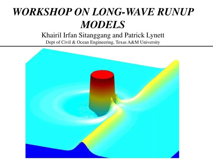
WORKSHOP ON LONG-WAVE RUNUP MODELS Khairil Irfan Sitanggang and Patrick Lynett Dept of Civil & Ocean Engineering, Texas A&M University. Governing Equations and Setup. z. x. z. a o. h o. h. H = h + z. e = a/h o m = (h o /l o ). l o. Governing Equations – Highly Nonlinear Boussinesq.

E N D
WORKSHOP ON LONG-WAVE RUNUP MODELSKhairil Irfan Sitanggang and Patrick LynettDept of Civil & Ocean Engineering, Texas A&M University
Governing Equations and Setup z x z ao ho h H = h + z e = a/ho m = (ho/lo) lo
Governing Equations – Highly Nonlinear Boussinesq Continuity Equation (Dimensionless)
Governing Equations – Highly Nonlinear Boussinesq Momentum Equation (Dimensionless)
Numerical Algorithm • Predictor - Corrector Scheme • 3rd-order explicit Adams-Bashforth (Press et al., 1989) predictor step - (Dt)3 • 4th -order implicit Adams-Moulton corrector step - (Dt)4 • Finite difference spatial derivatives to 4th-order accuracy - (Dx)4 • Scheme developed to solve the Boussinesq equations in 2HD • Not a computationally efficient solver for the NLSW equations or 1HD setups
Practical Simulation • Bottom friction based on the quadratic friction law • Wave breaking with an eddy viscosity model Comparison with data from Hansen & Svendsen (1979) • Runup/rundown uses the extrapolation moving shoreline procedure (Lynett et al, 2002)
Linear extrapolation- imaginary points in dry region Moving Boundary Algorithm • The underlying assumption is that very near the wet-dry boundary, the wave is linear in slope: • The free surface and velocity are linearly extrapolated through the wet-dry boundary, creating “imaginary” points in the dry region. • Wet nodal points near the wet-dry boundary use the extrapolated points when calculating finite difference derivates (5-point centered differences)
t1 t2 t4 t3 t6 t5 t7 t8 Validation of Runup algorithm • Runup of solitary waves • Comparison with experimental data taken from Synolakis (1987) • Numerical simulation parameters: • Wave height / water depth = 0.04 • Beach slope = 1:20 • Comparison with experimental data: Numerical results Experimental data
Validation of Runup algorithm Inundation comparisons • Runup of solitary wave around a circular island • Experimental data taken from Liu et al. (1995) Black dots represent the maximum experimental runup, while the light red shows the inundated area
Benchmark #1 • Initial free surface given • Run with: • NLSW • Boussinesq • Will examine the dispersive effect & required grid resolution near shoreline for numerical convergence • Simulations have no bottom friction, wave breaking not included
Benchmark #1 • Numerical convergence • Nearshore grid ~1.5 m is required for numerical convergence • Error much larger in velocity predictions
Benchmark #1 • CPU requirements: • Numerical model uses a constant dx and dt • dt is chosen based on a Courant formulation, where the characteristic velocity is the long wave velocity in the deepest water depth in the domain. • With constant slope to offshore boundary (and very deep water) a small time step is required. • NLSW simulation: • dx=1.5 m, dt=0.0018 s • nx~32,000, nt~170,000 (endx~50 km, endt~300s) • 51 MB of RAM • 40 hrs of CPU time on a 1.8 Ghz desktop! • ~0.9 seconds per time step • Numerical implementation not developed for large 1HD problems or NLSW equations
Benchmark #1 • NLSW numerical result matches solution very well • Boussinesq solution indicates that dispersive effects during shoaling may play a significant role • Shoreline elevation and velocity time histories Boussinesq numerical vs NLSW numerical vs Analytical
Benchmark #1 • Snapshots of free surface and velocity at various times
Benchmark #1 • Conclusions • Required small grid for convergent runup results leads to very large CPU times for a 1HD problem • Large grid error more significant for velocity comparisons • NLSW numerical results match well for both shoreline and spatial profiles • Boussinesq predicts higher maximum runup, but lower maximum speeds • Frequency dispersion may be important during shoaling, as the wave becomes very steep
Benchmark #2 Khairil Irfan Sitanggang, Patrick LynettDept of Civil & Ocean Engineering, Texas A&M University, U.S.AAlejandro OrfilaIMEDEA (CSIC-UIB), Spain • CPU requirements: • Numerical model uses a constant dx and dt • To capture the oscillations inside the cove, a relatively small global grid size was used • Boussinesq simulation: • dx~0.012 m, dt~0.005 s • nx~450, ny~300, nt~4,500 (endt=25s) • 200 MB of RAM • 5.5 hrs of CPU time on a 1.8 Ghz desktop • ~4.5 seconds per time step • Tsunami generation by internal source generator, using specified input wave time series
Benchmark #2 • Tsunami Approach on Complex Bathymetry • Bottom friction included (quadratic friction law) • Friction coefficient = 0.0025 • Breaking model used • Wave begins to “break” when zt>0.65[g(h+z)]0.5 • Energy dissipation (eddy viscosity model) is added at the breaking locations
Benchmark #2 • Tsunami Approach on Complex Bathymetry • Animation from Boussinesq simulation (wide view)
Benchmark #2 • Tsunami Approach on Complex Bathymetry • Animation from Boussinesq simulation (shoreline closeup) • Max predicted runup in cove ~ 6.5 cm.
Benchmark #2 • Tsunami Approach on Complex Bathymetry • Comparison w/ video data • Angle of approach of the positive wave is different, leading to different runup patterns
Benchmark #2 • Free surface time series comparisons
Benchmark #2 • Conclusions • Model does an OK job at recreating the experiment • Primary differences due to different approach angle of the positive wave • Possible causes: • Breaking not predicted correctly • Bottom friction underestimated • Input wave not exact • No significant differences between NLSW and Boussinesq for this case
Benchmark #3 Khairil Irfan Sitanggang, Patrick LynettDept of Civil & Ocean Engineering, Texas A&M University, U.S.A • CPU requirements: • Case A: • dx=10 m, dt=0.16 s (small dt for deep water stability) • nx=470, nt=450 • Boussinesq CPU time= 35 seconds on 1.8 Ghz desktop • Case B: • dx=0.25 m, dt=0.008 s • nx=400, nt=1400 • Boussinesq CPU time= 90 seconds on 1.8 Ghz desktop • For reference, numerical integration of the analytical solution required: • nx=1300, nt=2000 • CPU time = 6 hours on 1.8 Ghz desktop (lots of integration with Bessel & exponential functions)
Benchmark #3 • Subaerial slide • Animation of Case A from Boussinesq Simulation No bottom friction Breaking model not implemented Slide is shown as the yellow area Slide very thin
Benchmark #3 • CASE A comparisons (large tanb/m)
Benchmark #3 • Subaerial slide • Animation of Case B from Boussinesq Simulation No bottom friction Breaking model not implemented
Benchmark #3 • CASE B comparisons (small tanb/m)
Benchmark #3 • Conclusions • Case A: • Except for very early time, agreement excellent • Shoreline does not move much • NLSW and Boussinesq identical • Case B: • Agreement with analytical solution OK at early time, but differences grow quickly • The analytical solution, due to assumptions on the slide forcing, is not adequate for this case • Some difference between NLSW and Boussinesq at later times, but relatively minor • Indications that turbulence and/or dispersive effects become important at later times