Download
1 / 25
260 likes | 463 Views
Clock Synchronization in Sensor Networks*. * Timing-sync Protocol for Sensor Networks (SenSys 2003) Saurabh Ganeriwal, Ram Kumar & Mani B. Srivastava * Fine-Grained Network Time Synchronization using Reference Broadcasts Jeremy Elson, Lewis Girod & Deborah Estrin ( OSDI 2002 ). Introduction.

E N D
Clock Synchronization in Sensor Networks* *Timing-sync Protocol for Sensor Networks (SenSys 2003) Saurabh Ganeriwal, Ram Kumar & Mani B. Srivastava *Fine-Grained Network Time Synchronization using Reference Broadcasts Jeremy Elson, Lewis Girod & Deborah Estrin (OSDI 2002)
Introduction • Sensor nodes maintain local clocks • Typically lower precision clocks (crystal oscillators) • Clocks need to be synchronized to determine • Exact timing of events • Chronology of events • Clock synchronization • Global : all nodes are synchronized to a single clock • Example: NTP (often used in LANS) • Local : a set of “ localized” nodes are synchronized • Reference Broadcast Synchronization (RBS) • Post-facto Synchronization
Challenges • Scalability • Must be scalable to a large number of nodes • Energy Efficiency • Limited messaging • GPS technology cannot be employed • Requirements are more stringent • Microsecond precision desirable • Local : a set of “ localized” nodes are synchronize • Clock skew is large • Two node clocks might drift 1–100µsec per second
Clock Synchronization Models • Maintain relative notion of time • Generate the right chronology of events • Clocks need not be synchronized • Relative Clocks • Nodes maintain individual clocks • Maintain relative drift information with other clocks • RBS • “Always On” Model • Every clock is synchronized to a reference clock • Superset of the above models • TSPN
Today’s Talk • TSPN : Time-Sync Protocol for Sensor Networks • Sender-Receiver synchronization (classical approach) • needs MAC level integration • Always-On • RBS : Reference Broadcast Synchronization • Receiver-Receiver synchronization • Could be implemented at user-level • Relative Sync
Packet Delay (Uncertainty) Model • Sender Uncertainty • Send, Access, Transmission • Propagation Uncertainty • Negligible • Speed thru medium = 1foot/nanosecond = c • Receiver Uncertainty • Packet reception • Packet processing
TSPN • Clock Sync Algorithm involves 2 steps • Level Discovery phase • Synchronization phase • TSPN makes the following assumptions • Sensor nodes have unique identifiers • Node is aware of its neighbors • Bi-directional links • Creating the hierarchical tree is not exclusive to TSPN
TSPN: Level Discovery • Algorithm • Root node is assigned level i = 0 • broadcasts “level discovery pkt.” • Neighbors get packet and assign level i+1 to themselves • Ignore discovery pkts. once level has been assigned • Broadcast “level discovery pkt.” with own level • STOP when all nodes have been assigned a level • Optimization • Use minimum spanning trees instead of flooding
Level # Value of T1 Level # T1, T2, T3 TSPN: Synchronization phase • Synchronization using handshake between a pair of nodes (sender-initiated) • Assuming no clock drift and propagation delay do not change Clock drift Delay • A can now synchronize with B
TSPN: Synchronization • Algorithm • Root node initiates the protocol • broadcasts “time sync pkt.” • Nodes at level = 1 • Wait for a random time, initiate time-sync with root • On receiving ACK .. Synchronize with root • Nodes at level = 2 overhear sync from nodes at level 1 • Do a random back-off, initiate time-sync with level 1 node • Nodes sends ACK only if it has been synchronized • If a node does not receive an ACK, resend time-sync pulse after a timeout.
RBS: Reference Broadcast Synchronization • Eliminate “non-deterministic latency at the sender • NIC delay • Protocol processing • Critical path length reduced • Packets do not need to store explicit timing information • Relative time synchronization RBS
RBS: How it Works? • Characterize Receiver Error • Determine Phase Offset between nodes • Determine Clock Skew between nodes • Empirically determined • With knowledge of phase offset and clock skew, the clocks of any two nodes can be synchronized
RBS: Receiver Error Characterization Histogram showing the distribution of inter-receiver phase offsets recorded for 1,478 broadcast packets, grouped into 1µsec buckets. The curve is a plot of the best-fit Gaussian parameters. (µ = 0;s = 11:1µsec, confidence=99.8%) Accuracy can be increased by increasing the number of sync messages
RBS: Phase Offset Estimation Analysis of expected group dispersion (i.e., maximum pair-wise error) after reference-broadcast synchronization. Each point represents the average of 1,000 simulated trials. The underlying receiver is assumed to report packet arrivals with error conforming to last figure. Mean group dispersion, and standard deviation from the mean, for a 2-receiver (bottom) and 20-receiver (top) group.
RBS: Phase Offset with Skew Each point represents the phase offset between two nodes as implied by the value of their clocks after receiving a reference broadcast. A node can compute a least-squared error fit to these observations (diagonal line), and convert time values between its own clock and that of its peer. Synchronization of the Mote’s internal clock
RBS: Multi-hop Time Synchronization Example, we can compare the time of E1(R1) with E10(R10) by transforming E1(R1) ►E1(R4) ► E1(R8) ► E1(R10). Conversions can be made automatically by using the shortest path algorithm
Level # Value of T1 Level # T1, T2, T3 Error Analysis: TPSN & RBS • Analyze sources of error for the algorithms • Compare TPSN and RBS • Trade-Offs Clock drift
Error Analysis: TPSN Drift between A & B
Error Analysis: TPSN By rearranging the terms, we get
Error Comparison: TPSN & RBS TPSN RBS • Comparison/Discussion: • Sender delays • Receiver delays • Relative Skews