Download
1 / 32
330 likes | 799 Views
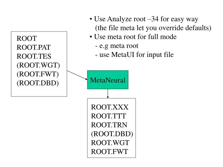
Use Analyze root –34 for easy way (the file meta let you override defaults) Use meta root for full mode - e.g meta root - use MetaUI for input file. ROOT ROOT.PAT ROOT.TES (ROOT.WGT) (ROOT.FWT) (ROOT.DBD). MetaNeural. ROOT.XXX ROOT.TTT ROOT.TRN (ROOT.DBD) ROOT.WGT

E N D
Use Analyze root –34 for easy way • (the file meta let you override defaults) • Use meta root for full mode • - e.g meta root • - use MetaUI for input file ROOT ROOT.PAT ROOT.TES (ROOT.WGT) (ROOT.FWT) (ROOT.DBD) MetaNeural ROOT.XXX ROOT.TTT ROOT.TRN (ROOT.DBD) ROOT.WGT ROOT.FWT
S S S S S • ANALYZE = MetaNeural Alternative Code • Either run meta root analyze root.pat –34 (single training and testing) analyze root.pat –3434 (LOO) analyze root.txt 34 (bootstrap mode) • Results for analyze are in resultss.xxx and resultss.ttt • Results from MetaNeural are in root.xxx and root.ttt • MetaNeural input file is generated automatically in analyze • The file name meta overrides the default input file for analyze
MetaNeural Input File for the ROOT 4 => 4 layers 2 => 2 inputs 16 => # hidden neurons in layer #1 4 => # hidden neurons in layer# 2 1 => # outputs 300 => epoch length (hint:always use 1, for the entire batch) 0.01 => learning parameters by weight layer (hint: 1/# patterns or 1/# epochs) 0.01 0.01 0.5 => momentum parameters by weight layer (hint use 0.5) 0.5 0.5 10000000 => some very large number of training epochs 200 => error display refresh rate 1 =>sigmoid transfer function 1 => Temperature of sigmoid check.pat => name of file with training patterns (test patterns in root.tes) 0 => not used (legacy entry) 100 => not used (legacy entry) 0.02000 => exit training if error < 0.02 0 => initial weights from a flat random distribution 0.2 => initial random weights all fall between –2 and +2
EXAMPLE DATA SETS • IRIS data • Checkerboard data • Svante wold’s QSAR data • Cherkassky’s nonlinear function • Albumin QSAR data
FILES RELATED TO CHECKERBOARD EXAMPLE CHECK_NET.BAT CHECK_DATA.BAT CHECK_TEST.BAT CHECK.PAT
QSAR DATA SET EXAMPLE: 19 Amino Acids From Svante Wold, Michael Sjölström, Lennart Erikson, "PLS-regression: a basic tool of chemometrics," Chemometrics and Intelligent Laboratory Systems, Vol 58, pp. 109-130 (2001) RENSSELAER
PLS 1 latent variable
PLS 1 latent variable No aromatic AAs
1 latent variable Gaussian Kernel PLS (sigma = 1.3) With aromatic AAs
Chemoinformatic Models to Predict Binding Affinities to Human Serum Albumin:G. Colmenarejo et. al., J. Med. Chem 2001, 44, pp. 4370-4378 95 Molecules Widely different compounds 250-1500+ Descriptors
Binding affinities to human serum • albumin (HSA): log K’hsa • Gonzalo Colmenarejo, GalaxoSmithKline • J. Med. Chem. 2001, 44, 4370-4378 • 95 molecules, 250-1500+ descriptors • Widely different compounts
Histograms PIP (Local Ionization Potential) Wavelet Coefficients Electron Density-Derived TAE-wavelet Descriptors 1 ) Surface properties are encoded on 0.002 e/au3 surface Breneman, C.M. and Rhem, M., J. Comp. Chem., 1997,18(2), p. 182-197 2 ) Histograms or wavelet encoded of surface properties give TAE property descriptors
PEST-Shape Descriptors: Surface Property-Encoded Ray Tracing • TAE Internal Ray Reflection - low resolution scan Isosurface (portion removed) with 750 segments RENSSELAER
Shape-Aware Molecular Descriptors from Property/Segment-Length Distributions • Segment length and point-of-incidence value form 2D-histogram • Each bin of 2D-histogram becomes a hybrid descriptor • 36 descriptors per hybrid length-property PIP vs Segment Length RENSSELAER
CHERKASSKY’S NONLINEAR BENCHMARK DATA • Generate 500 datapoints (400 training; 100 testing) for: Cherkas.bat
Y=sin|x|/|x| • Generate 500 datapoints (100 training; 500 testing) for:
Comparison Kernel-PLS with PLS 4 latent variables sigma = 0.08 PLS Kernel-PLS