Download

1 / 83
861 likes | 1.12k Views
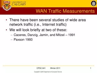
Traffic Measurements. Modified from Carey Williamson. Network Traffic Measurement. A focus of networking research for 20+ years Collect data or packet traces showing packet activity on the network for different applications Study, analyze, characterize Internet traffic Goals:

E N D
Traffic Measurements Modified from Carey Williamson
Network Traffic Measurement • A focus of networking research for 20+ years • Collect data or packet traces showing packet activity on the network for different applications • Study, analyze, characterize Internet traffic • Goals: • Understand the basic methodologies used • Understand the key measurement results to date
Why Network Traffic Measurement? • Understand the traffic on existing networks • Develop models of traffic for future networks • Useful for simulations, capacity planning studies
Measurement Environments • Local Area Networks (LAN’s) • e.g., Ethernet LANs • Wide Area Networks (WAN’s) • e.g., the Internet • Wireless LANs • …
Requirements • Network measurement requires hardware or software measurement facilities that attach directly to network • Allows you to observe all packet traffic on the network, or to filter it to collect only the traffic of interest • Assumes broadcast-based network technology, superuser permission
Measurement Tools (1 of 3) • Can be classified into hardware and software measurement tools • Hardware: specialized equipment • Examples: HP 4972 LAN Analyzer, DataGeneral Network Sniffer, others... • Software: special software tools • Examples: tcpdump, xtr, SNMP, others...
Measurement Tools (2 of 3) • Measurement tools can also be classified as active or passive • Active: the monitoring tool generates traffic of its own during data collection (e.g., ping, pchar) • Passive: the monitoring tool is passive, observing and recording traffic info, while generating none of its own (e.g., tcpdump)
Measurement Tools (3 of 3) • Measurement tools can also be classified as real-time or non-real-time • Real-time: collects traffic data as it happens, and may even be able to display traffic info as it happens, for real-time traffic management • Non-real-time: collected traffic data may only be a subset (sample) of the total traffic, and is analyzed off-line (later), for detailed analysis
Potential Uses of Tools (1 of 4) • Protocol debugging • Network debugging and troubleshooting • Changing network configuration • Designing, testing new protocols • Designing, testing new applications • Detecting network weirdness: broadcast storms, routing loops, etc.
Potential Uses of Tools (2 of 4) • Performance evaluation of protocols and applications • How protocol/application is being used • How well it works • How to design it better
Potential Uses of Tools (3 of 4) • Workload characterization • What traffic is generated • Packet size distribution • Packet arrival process • Burstiness • Important in the design of networks, applications, interconnection devices, congestion control algorithms, etc.
Potential Uses of Tools (4 of 4) • Workload modeling • Construct synthetic workload models that concisely capture the salient characteristics of actual network traffic • Use as representative, reproducible, flexible, controllable workload models for simulations, capacity planning studies, etc.
Traffic Measurement Time Scales • Performance analysis • representative models • throughput, packet loss, packet delay • Microseconds to minutes • Network engineering • network configuration • capacity planning • demand forecasting • traffic engineering • Minutes to years • Different measurement methods
Properties • Most basic view of traffic is as a collection of packets passing through routers and links • Packets and Bytes • One can capture/observe packets at some location • Packet arrivals • interarrivals • count traffic at timescale T • Captures workload generated by traffic on a per-packet basis • Packet Size • time series of Byte count • Captures the amount of consumed bandwidth • packet size distribution • router design etc.
Higher-level Structure • Transport protocols and applications • ON/OFF process • bursty workload • Packet-level • Packet Train • interarrival threshold • Session • single execution of an application • Human generated
Flows • Set of packets passing an observation point during a time interval with all packets having a set of common properties • Header field contents, packet characteristics, etc. • IP flows • source/destination addresses • IP or transport header fields • prefix • Network-defined flow • network’s workload • ingress and egress • Traffic matrix and Path matrix
Semantically Distinct Traffic Types • Control Traffic • Control plane • Routing protocols • BGP, OSPF, IS-IS • Measurement and management • SNMP • General control packets • ICMP • Data plane • Malicious Traffic
Challenges • Practical issues • Observability • Core simplicity • Flows • Packets • Distributed Internetworking • IP Hourglass • Data volume • Data sharing
Challenges • Statistical difficulties • Long tails and High variability • Instability of metrics • Modeling difficulty • Confounding intuition • Stationarity and stability • Stationarity: joint probability distribution does not change when shifted in time • Stability: consistency of properties over time • Autocorrelation and memory in system behavior • High dimensionality
Tools • Packet Capture • General purpose systems • libpcap • tcpdump • ethereal • scriptroute • … • Special purpose system • Control plane traffic • GNU Zebra • Routeviews
Data Management • Full packet capture and storage is challenging • Limitations of commodity PC • Data stream management • Big Data platforms • Hadoop, etc.
Data Reduction • Lossy compression • Counters • SNMP Management Information Base • Flow capture • Packet trains • Packet flows
Data Reduction • Sampling • Basic packet sampling • Random: with fixed probability • Deterministic: periodic samples • Stratified: multi step sampling • Trajectory sampling • Chose a randomly sampled packet at all locations
Data Reduction • Summarization • Bloom filters • Sketches: Dimension reducing random projections • Probabilistic counting • Landmark/sliding window models
Review: Bloom Filters • Given a set S = {x1,x2,x3,…xn} on a universe U, want to answer queries of the form: • Bloom filter provides an answer in • “Constant” time (time to hash). • Small amount of space. • But with some probability of being wrong. • Alternative to hashing with interesting tradeoffs.
B 0 0 0 0 0 0 0 0 0 0 0 0 0 0 0 0 B 0 1 0 0 1 0 1 0 0 1 1 1 0 1 1 0 B 0 1 0 0 1 0 1 0 0 1 1 1 0 1 1 0 B 0 1 0 0 1 0 1 0 0 1 1 1 0 1 1 0 Review: Bloom Filters Start with an m bit array, filled with 0s. Hash each item xjin S k times. If Hi(xj) = a, set B[a] = 1. To check if y is in S, check B at Hi(y). All k values must be 1. Possible to have a false positive; all k values are 1, but y is not in S. n items m= cn bits k hash functions
Review: Bloom Filters • Tradeoffs • Three parameters. • Size m/n : bits per item. • Time k : number of hash functions. • Error f : false positive probability.
Review: Bloom Filters • False Positive Probability • Pr(specific bit of filter is 0) is • If r is fraction of 0 bits in the filter then false positive probability is • Approximations valid as r is concentrated around E[r]. • Martingale argument suffices. • Find optimal at k = (ln 2)m/n by calculus. • So optimal fpp is about (0.6185)m/n n items m= cn bits k hash functions
Data Reduction • Dimensionality reduction • Clustering • Principal Component Analysis • Probabilistic models • Distribution models • Dependence structure • Inference • Traffic Matrix estimation
Curse of Dimensionality. • A major problem is the curse of dimensionality. • If the data x lies in high dimensional space, then an enormous amount of data is required to learn distributions or decision rules. • Example: 50 dimensions. Each dimension has 20 levels. This gives a total of cells. But the no. of data samples will be far less. There will not be enough data samples to learn.
Dimension Reduction • One way to avoid the curse of dimensionality is by projecting the data onto a lower-dimensional space. • Techniques for dimension reduction: • Principal Component Analysis (PCA) • Fisher’s Linear Discriminant • Multi-dimensional Scaling. • Independent Component Analysis. • …
Principal Component Analysis • PCA is the most commonly used dimension reduction technique. • Also called the Karhunen-Loeve transform • PCA – data samples • Compute the mean • Computer the covariance:
Compute the eigenvalues and eigenvectors of the matrix Solve Order them by magnitude: PCA reduces the dimension by keeping direction such that Principal Component Analysis
For many datasets, most of the eigenvalues \lambda are negligible and can be discarded. Principal Component Analysis The eigenvalue measures the variation In the direction e Example:
Why Principal Component Analysis? • Motive • Find bases which has high variance in data • Encode data with small number of bases with low MSE
Dimensionality Reduction Can ignore the components of less significance. You do lose some information, but if the eigenvalues are small, you don’t lose much • n dimensions in original data • calculate n eigenvectors and eigenvalues • choose only the first p eigenvectors, based on their eigenvalues • final data set has only p dimensions
Variance Dimensionality Dimensionality Reduction
PCA may not find the best directions for discriminating between two classes. Example: suppose the two classes have 2D Gaussian densities as ellipsoids. 1st eigenvector is best for representing the probabilities. 2nd eigenvector is best for discrimination. PCA and Discrimination
Principal Component Analysis (PCA) Linear methods.. One Dimensional Manifold
Nonlinear Manifolds.. PCA and MDS see the Euclidean distance A What is important is the geodesic distance Unroll the manifold
To preserve structure preserve the geodesic distance and not the euclidean distance.
Two methods • Tenenbaum et.al’s Isomap Algorithm • Global approach. • On a low dimensional embedding • Nearby points should be nearby. • Farway points should be faraway. • Roweis and Saul’s Locally Linear Embedding Algorithm • Local approach • Nearby points nearby
Isomap • Estimate the geodesic distance between faraway points. • For neighboring points Euclidean distance is a good approximation to the geodesic distance. • For farway points estimate the distance by a series of short hops between neighboring points. • Find shortest paths in a graph with edges connecting neighboring data points Once we have all pairwise geodesic distances use classical metric MDS
Isomap - Algorithm • Determine the neighbors. • All points in a fixed radius. • K nearest neighbors • Construct a neighborhood graph. • Each point is connected to the other if it is a K nearest neighbor. • Edge Length equals the Euclidean distance • Compute the shortest paths between two nodes • Floyd’s Algorithm • Djkastra’s ALgorithm • Construct a lower dimensional embedding. • Classical MDS