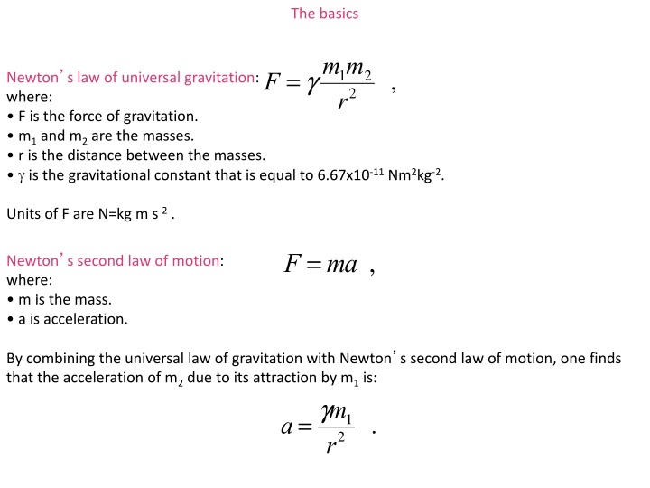
Newton ’ s law of universal gravitation : where: F is the force of gravitation.

The basics • Newton’s law of universal gravitation: • where: • F is the force of gravitation. • m1 and m2 are the masses. • r is the distance between the masses. •  is the gravitational constant that is equal to 6.67x10-11 Nm2kg-2. • Units of F are N=kg m s-2 . • Newton’s second law of motion: • where: • m is the mass. • a is acceleration. • By combining the universal law of gravitation with Newton’s second law of motion, one finds that the acceleration of m2 due to its attraction by m1 is:

The basics • Gravitational acceleration is thus: • where: • ME is the mass of the Earth. • RE is the Earth’s radius. • Units of acceleration are m s-2, or gal=0.01 m s-2. • The Earth is an oblate spheroid that is fatter at the equator and is thinner at the poles. • There is an excess mass under the equator. • Centrifugal acceleration reduces gravitational attraction. Thus, the further you are from the rotation axis, the greater the centrifugal acceleration is.

The basics From: http://principles.ou.edu/earth_figure_gravity/geoid/

The basics • g is a vector field: • where r is a unit vector pointing towards the earth’s center. The gravitational potential, U, is a scalar field: • Note that Earth’s gravitational potential is negative. • Potentials are additive, and this property makes them easier (than vectors) to work with. • To verify that U is the potential field of g take its derivative with respect to R. • The gradient of a scalar field is a vector field.

Surface gravity anomalies due to some buried bodies x/z z a The general equation is: where:  is the gravitational constant  is the density contrast r is the distance to the observation point a is the angle from vertical V is the volume Question: Why a cosine term? Solution for a sphere:

Surface gravity anomalies due to some buried bodies Infinitely long horizontal cylinder:

Surface gravity anomalies due to some buried bodies Buried infinite slab:

Surface gravity anomalies due to some buried bodies An infinitely long horizontal cylinder The expression for a horizontal cylinder of a radius a and density : It is interesting to compare the solution for cylinder with that of a sphere. This highlights the importance of a 2-D gravity survey. cylinder sphere

Surface gravity anomalies due to some buried bodies What should be the spatial extent of the surveyed region? To answer this question it is useful to compute the anomaly half-distance, X1/2, i.e. the distance from the anomaly maximum to it’s medium. For a sphere, we get: • The signal due to a sphere buried at a depth Z can only be well resolved at distances out to 2-3 Z. • Thus, to resolve details of density structures of the lower crust (say 20-40 km), gravity measurements must be made over an extensive area.

The ambiguity of surface gravity anomalies In the preceding slide we have looked at the result of a forward modeling also referred to as the direct problem: In practice, however, the inverse modeling is of greater importance: Question: Can the data be inverted to obtain the density, size and shape of a buried body? • Inspection of the solution for a buried sphere reveals a non-uniqueness of that problem. The term a3 introduces an ambiguity to the problem, and different combinations of densities and radiican produce identical anomalies.

The ambiguity of surface gravity anomalies • The same gravity anomaly may be explained by different anomalous bodies, having different shapes and located at different depths: measured gravity anomaly Near surface very elongated body Shallow elongated body Deep sphere In summary, we want to know: But actually, gravity anomaly alone cannot provide this information.

The ambiguity of surface gravity anomalies Here’s an example from a Mid-Atlantic Ridge (MAR). The observed anomaly may be explained equally well with deep models with small density contrast or shallow models with greater density contrast. Question: is the MAR in isostatic equilibrium?

The geoid • Geoid • the observed equipotential surface that defines the sea level. • the shape a fluid Earth would have if it had exactly the gravity field of the Earth • roughly the sea-level surface - dynamic effects such as waves, and tides, must be excluded • geoid on continents lies below continents - corresponds to level of nearly massless fluid if narrow channels were cut through continents • geoid highs are gravity highs The vector gravity (g) is perpendicular to the geoid.

The geoid Reference geoid is a mathematical formula describing a theoretical equipotential surface of a rotating (i.e., centrifugal effect is accounted for) symmetric spheroidal earth model having realistic radial density distribution. observed geoid reference geoid The international gravity formula gives the theoretical gravitational acceleration on a reference geoid:

The geoid The geoid height anomaly is the difference in elevation between the measured geoid and the reference geoid. Note that the geoid height anomaly is measured in meters.

Geoid anomaly Map of geoid height anomaly: Figure from: www.colorado.edu/geography • Note that: • The differences between observed geoid and reference geoid are as large as 100 meters • In continental regions, they do not correlate with topography because of isostatic compensation Question: what gives rise to geoid anomaly?

Geoid anomaly • Differences between geoid and reference geoid are due to: • Topography • Density anomalies at depth Figure from Fowler

Geoid anomaly downwelling upwelling Flow Temp. What is the effect of mantle convection on the geoid anomaly? Two competing effects: Upwelling brings hotter and less dense material, the effect of which is to reduce gravity. Upwelling causes topographic bulge, the effect of which is to increase gravity. Figure from McKenzie et al., 1980

Geoid anomaly SEASAT provides water topography Note that the most prominent features on most geoid maps (depending on filtering used) are subductionzones.

Geoid anomaly Cross-sections across subduction-zone geoid anomalies show an asymmetric anomaly low (trench) and an anomaly high (presence of cold, dense slab in lighter asthenospere): Free-air gravity anomaly from satellite altimetry for the Tonga-Kermadec region Comparison of topography along east west profiles across the subduction zone at 20, 25 and 30°S (thick/blue) to observed topography (thin/black) (From: Billen and Gurnis, EPSL, 2001)

Geoid anomaly GEOID99: a refined model of the geoid in the United States Heights range from a low of -50.97 meters (magenta) in the Atlantic Ocean to a high of 3.23 meters (red) in the Labrador Strait

Geoid anomaly A model for mass change due to post-glacial rebound and the reloading of the ocean basins with seawater. Blue and purple areas indicate rising due to the removal of the ice sheets. Yellow and red areas indicate falling as mantle material moved away from these areas in order to supply the rising areas, and because of the collapse of the forebulges around the ice sheets.

Geoid anomaly and corrections • Geoid anomaly contains information regarding the 3-D mass distribution. But first, a few corrections should be applied: • Free-air (required) • Bouguer (required) • Terrain (optional)

Geoid anomaly and corrections Free-air correction, gFA: This correction accounts for the fact that the point of measurement is at elevation H, rather than at the sea level on the reference spheroid.

Geoid anomaly and corrections • Since: • where: •  is the latitude • h is the topographic height • g() is gravity at sea level • R() is the radius of the reference spheroid at  • The free-air correction is thus: • This correction amounts to 3.1x10-6 ms-2 per meter elevation. Question: should this correction be added or subtracted? The free-air anomaly is the geoid anomaly, with the free-air correction applied:

Geoid anomaly and corrections

Geoid anomaly and corrections Bouguer correction, gB: This correction accounts for the gravitational attraction of the rocks between the point of measurement and the sea level.

Geoid anomaly and corrections An infinite horizontal slab of finite thickness: Setting (y)= c and integration with respect to r from zero to infinity and with respect to y between 0 and h leads to: Note that the gravity anomaly caused by an infinite horizontal slab of thickness h and density c is independent of its distance b from the observer.

Geoid anomaly and corrections

Geoid anomaly and corrections The Bouguer correction is: where:  is the universal gravitational constant  is the rock density h is the topographic height For rock density of 2.7x103 kgm-3, this correction amounts to 1.1x10-6 ms-2 per meter elevation. Question: should this correction be added or subtracted? The Bouguer anomaly is the geoid anomaly, with the free-air and Bouguer corrections applied:

Geoid anomaly and corrections Terrain correction, gT: This correction accounts for the deviation of the surface from an infinite horizontal plane. The terrain correction is small, and except for area of mountainous terrain, can often be ignored.

Geoid anomaly and corrections The Bouguer anomaly including terrain correction is: • Bouguer anomaly for offshore gravity survey: • Replace water with rock • Apply terrain correction for seabed topography After correcting for these effects, the ''corrected'' signal contains information regarding the 3-D distribution of mass in the earth interior.

Isostasy The deflection of plumb-bob near mountain chains is less than expected. Calculations show that the actual deflection may be explained if the excess mass is canceled by an equal mass deficiency at greater depth. A plumb-bob Picture from wikipedia

Isostasy: the Airy hypothesis (application of Archimedes’ principal) h1 d u r3 r1 s • Two densities, that of the rigid upper layer, u, and that of the substratum, s. • Mountains therefore have deep roots. A mountain height h1 is underlain by a root of thickness: • Ocean basin depth, h2, is underlain by an anti-root of thickness:

Isostasy: the Pratt’s hypothesis • The depth to the base of the upper layer is constant. • The density of rocks beneath mountains is less than that beneath valleys. • A mountain whose height is h1 is underlain by a root whose density 1 is: • Ocean basin whose depth is h2 is underlain by a high density material, 2, that is given by:

Isostasy:

Isostasy • Questions: • Which is the correct hypothesis? • Does isostatic equilibrium apply everywhere? • Is the person resting on top of a spring-mattress in a state of isostatic equilibrium?

Isostasy: elastic flexure Like the springs inside the mattress, the elastic lithosphere can also support excess mass. Thick plates can support more excess mass than thin plates.

Isostasy: elastic flexure The response of the lithosphere to a vertical load depends on the lithosphere elastic properties as follows: where D is the flexural rigidity, that is given by: with: E being Young Modulus h being the plate thickness  being Poisson’s ratio

Isostasy: elastic flexure The figure below shows the solution for the case of a line load: Figure from Fowler Note the flexural bulge on either side of the depression. Of course in reality the boundary conditions are more complex…

Isostasy: example from the Hawaii chain free-air bathymetry • Two effects: • Elastic flexure due to island load. • A swell due to mantle upwelling. Figure from Fowler

Isostasy: example from the Mariana subduction zone deflection [km] distance [km] Fluxural bulge Figure from Fowler • The accretionary wedge loads the plate edge causing it to bend. • A flexural bulge is often observed adjacent to the trench. • Topography of Mariana bulge implies a 28 km thick plate.

Isostasy example from the Tonga subduction zone deflection [km] distance [km] Figure from Fowler • The Tonga slab bends more steeply than can be explained by an elastic model. • It turned out that an elastic-plastic model for the lithosphere can explain the bathymetry data.

Isostasy: local versus regional isostatic equilibrium According to Pratt and Airy hypotheses, excess mass is perfectly compensated everywhere. This situation is referred to as local isostasy. The situation where some of the load is supported by the strength of the lithosphere is referred to as regional isostasy. In this case, isostatic equilibrium occurs on a larger scale, but not at any point.

Isostasy Questions: Isostatic equilibrium means no excess mass. Does this mean no gravitational anomaly. Can we distinguish compensated from uncompensated topographies?

Isostasy: gravity 100% compensated A rule of thumb: A region is in isostatic equilibrium if the Bouguer anomaly is a mirror image of the topography. Figure from Fowler

Isostasy: gravity Uncompensated A rule of thumb: A region is NOT in isostatic equilibrium if the Bouguer anomaly remains flat under topographic highs and lows. Figure from Fowler

Isostasy: isostatic rebound The rate of isostatic rebound depends on the elastic properties of the lithosphere (including its thickness) as well as the mantle viscosity. Isostatic rebound can be observed if a large enough load has been added or removed fast enough. Figure from Fowler

Newton ’ s law of universal gravitation : where: F is the force of gravitation.