Download
1 / 75
770 likes | 931 Views
Congestion Overview (§ 6.3, § 6.5.10). Topic. Understanding congestion, a “traffic jam” in the network Later we will learn how to control it. What’s the hold up?. Network. Nature of Congestion. Simplified view of per port output queues

E N D
Congestion Overview (§6.3, §6.5.10)
Topic • Understanding congestion, a “traffic jam” in the network • Later we will learn how to control it What’s the hold up? Network CSE 461 University of Washington
Nature of Congestion • Simplified view of per port output queues • Typically FIFO (First In First Out), discard when full Router Router = Queued Packets (FIFO) Queue CSE 461 University of Washington
Nature of Congestion (2) • Queues help by absorbing bursts when input > output rate • But if input > output rate persistently, queue will overflow • This is congestion • Congestion is a function of the traffic patterns – can occur even if every link have the same capacity CSE 461 University of Washington
Effects of Congestion • What happens to performance as we increase the load? CSE 461 University of Washington
Effects of Congestion (2) • What happens to performance as we increase the load? CSE 461 University of Washington
Effects of Congestion (3) • As offered load rises, congestion occurs as queues begin to fill: • Delay and loss rise sharply with more load • Throughput falls below load (due to loss) • Goodput may fall below throughput (due to spurious retransmissions) • None of the above is good! • Want to operate network just before the onset of congestion CSE 461 University of Washington
Bandwidth Allocation • Important task for network is to allocate its capacity to senders • Good allocation is efficient and fair • Efficient means most capacity is used but there is no congestion • Fair means every sender gets a reasonable share the network CSE 461 University of Washington
Bandwidth Allocation (2) • Why is it hard? (Just split equally!) • Number of senders and their offered load is constantly changing • Senders may lack capacity in different parts of the network • Network is distributed; no single party has an overall picture of its state CSE 461 University of Washington
Bandwidth Allocation (3) • Key observation: • In an effective solution, Transport and Network layers must work together • Network layer witnesses congestion • Only it can provide direct feedback • Transport layer causes congestion • Only it can reduce offered load CSE 461 University of Washington
Bandwidth Allocation (4) • Solution context: • Senders adapt concurrently based on their own view of the network • Design this adaption so the network usage as a whole is efficient and fair • Adaption is continuous since offered loads continue to change over time CSE 461 University of Washington
Topic • What’s a “fair” bandwidth allocation? • The max-min fair allocation CSE 461 University of Washington
Recall • We want a good bandwidth allocation to be fair and efficient • Now we learn what fair means • Caveat: in practice, efficiency is more important than fairness CSE 461 University of Washington
Efficiency vs. Fairness • Cannot always have both! • Example network with traffic AB, BC and AC • How much traffic can we carry? B A C 1 1 CSE 461 University of Washington
Efficiency vs. Fairness (2) • If we care about fairness: • Give equal bandwidth to each flow • AB: ½ unit, BC: ½, and AC, ½ • Total traffic carried is 1 ½ units B A C 1 1 CSE 461 University of Washington
Efficiency vs. Fairness (3) • If we care about efficiency: • Maximize total traffic in network • AB: 1 unit, BC: 1, and AC, 0 • Total traffic rises to 2 units! B A C 1 1 CSE 461 University of Washington
The Slippery Notion of Fairness • Why is “equal per flow” fair anyway? • AC uses more network resources (two links) than AB or BC • Host A sends two flows, B sends one • Not productive to seek exact fairness • More important to avoid starvation • “Equal per flow” is good enough CSE 461 University of Washington
Generalizing “Equal per Flow” • Bottleneck for a flow of traffic is the link that limits its bandwidth • Where congestion occurs for the flow • For AC, link A–B is the bottleneck B A C 10 1 Bottleneck CSE 461 University of Washington
Generalizing “Equal per Flow” (2) • Flows may have different bottlenecks • For AC, link A–B is the bottleneck • For BC, link B–C is the bottleneck • Can no longer divide links equally … B A C 10 1 CSE 461 University of Washington
Max-Min Fairness • Intuitively, flows bottlenecked on a link get an equal share of that link • Max-min fair allocation is one that: • Increasing the rate of one flow will decrease the rate of a smaller flow • This “maximizes the minimum” flow CSE 461 University of Washington
Max-Min Fairness (2) • To find it given a network, imagine “pouring water into the network” • Start with all flows at rate 0 • Increase the flows until there is a new bottleneck in the network • Hold fixed the rate of the flows that are bottlenecked • Go to step 2 for any remaining flows CSE 461 University of Washington
Max-Min Example • Example: network with 4 flows, links equal bandwidth • What is the max-min fair allocation? CSE 461 University of Washington
Max-Min Example (2) • When rate=1/3, flows B, C, and D bottleneck R4—R5 • Fix B, C, and D, continue to increase A Bottleneck CSE 461 University of Washington
Max-Min Example (3) • When rate=2/3, flow A bottlenecks R2—R3. Done. Bottleneck Bottleneck CSE 461 University of Washington
Max-Min Example (4) • End with A=2/3, B, C, D=1/3, and R2—R3, R4—R5 full • Other links have extra capacity that can’t be used • , linksxample: network with 4 flows, links equal bandwidth • What is the max-min fair allocation? CSE 461 University of Washington
Adapting over Time • Allocation changes as flows start and stop Time CSE 461 University of Washington
Adapting over Time (2) Flow 1 slows when Flow 2 starts Flow 1 speeds up when Flow 2 stops Flow 3 limit is elsewhere Time CSE 461 University of Washington
Recall • Want to allocate capacity to senders • Network layer provides feedback • Transport layer adjusts offered load • A good allocation is efficient and fair • How should we perform the allocation? • Several different possibilities … CSE 461 University of Washington
Bandwidth Allocation Models • Open loop versus closed loop • Open: reserve bandwidth before use • Closed: use feedback to adjust rates • Host versus Network support • Who sets/enforces allocations? • Window versus Rate based • How is allocation expressed? TCP is a closed loop, host-driven, and window-based CSE 461 University of Washington
Additive Increase Multiplicative Decrease • AIMD is a control law hosts can use to reach a good allocation • Hosts additively increase rate while network is not congested • Hosts multiplicatively decrease rate when congestion occurs • Used by TCP • Let’s explore the AIMD game … CSE 461 University of Washington
AIMD Game • Hosts 1 and 2 share a bottleneck • But do not talk to each other directly • Router provides binary feedback • Tells hosts if network is congested Bottleneck 1 Host 1 Rest of Network 1 1 Router Host 2 CSE 461 University of Washington
AIMD Game (2) • Each point is a possible allocation Host 1 1 Congested Fair Optimal Allocation Efficient Host 2 0 1 CSE 461 University of Washington
AIMD Game (3) • AI and MD move the allocation Host 1 1 Congested Fair, y=x Additive Increase Optimal Allocation Multiplicative Decrease Efficient, x+y=1 Host 2 0 1 CSE 461 University of Washington
AIMD Game (4) • Play the game! Host 1 1 Congested Fair A starting point Efficient Host 2 0 1 CSE 461 University of Washington
AIMD Game (5) • Always converge to good allocation! Host 1 1 Congested Fair A starting point Efficient Host 2 0 1 CSE 461 University of Washington
AIMD Sawtooth • Produces a “sawtooth” pattern over time for rate of each host • This is the TCP sawtooth(later) Host 1 or 2’s Rate Multiplicative Decrease Additive Increase Time CSE 461 University of Washington
AIMD Properties • Converges to an allocation that is efficient and fair when hosts run it • Holds for more general topologies • Other increase/decrease control laws do not! (Try MIAD, MIMD, AIAD) • Requires only binary feedback from the network CSE 461 University of Washington
Feedback Signals • Several possible signals, with different pros/cons • We’ll look at classic TCP that uses packet loss as a signal CSE 461 University of Washington
TCP Tahoe/Reno • Avoid congestion collapse without changing routers (or even receivers) • Idea is to fix timeouts and introduce a congestion window (cwnd) over the sliding window to limit queues/loss • TCP Tahoe/Reno implements AIMD by adapting cwnd using packet loss as the network feedback signal CSE 461 University of Washington
TCP Tahoe/Reno (2) • TCP behaviors we will study: • ack clocking • Adaptive timeout (mean and variance) • Slow-start • Fast Retransmission • Fast Recovery • Together, they implement AIMD CSE 461 University of Washington
Sliding Window ACK Clock • Each in-order ack advances the sliding window and lets a new segment enter the network • acks “clock” data segments 20 19 18 17 16 15 14 13 12 11 Data Ack 1 2 3 4 5 6 7 8 9 10 CSE 461 University of Washington
Benefit of ACK Clocking • Consider what happens when sender injects a burst of segments into the network Queue Slow (bottleneck) link Fast link Fast link CSE 461 University of Washington
Benefit of ACK Clocking (2) • Segments are buffered and spread out on slow link Segments “spread out” Fast link Slow (bottleneck) link Fast link CSE 461 University of Washington
Benefit of ACK Clocking (3) • acks maintain the spread back to the original sender Slow link Acks maintain spread CSE 461 University of Washington
Benefit of ACK Clocking (4) • Sender clocks new segments with the spread • Now sending at the bottleneck link without queuing! Segments spread Queue no longer builds Slow link CSE 461 University of Washington
Benefit of ACK Clocking (4) • Helps the network run with low levels of loss and delay! • The network has smoothed out the burst of data segments • ack clock transfers this smooth timing back to the sender • Subsequent data segments are not sent in bursts so do not queue up in the network CSE 461 University of Washington