Download
1 / 12
260 likes | 1.04k Views
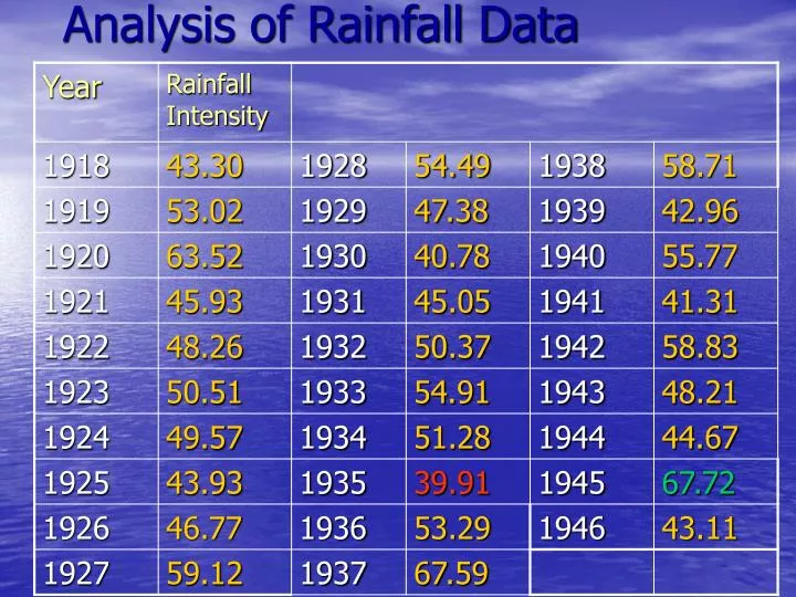
Analysis of Rainfall Data. 50.7. 59.4. Sample mean = Sample variance = S 2 = Approximately, 68% within 50.7 +/- 1 x 7.71 or 43.0 to 58.4 Approximately, 95% within 50.7 +/- 2 x 7.71 or 35.3 to 66.1. S = 7.71. Construction of Histogram. Rearrange data in increasing order

E N D
50.7 59.4 Sample mean = Sample variance = S2 = Approximately, 68% within 50.7+/- 1x7.71 or 43.0 to 58.4 Approximately, 95% within 50.7 +/- 2 x 7.71 or 35.3 to 66.1 S = 7.71
Construction of Histogram • Rearrange data in increasing order • Note the range and divide into suitable intervals (say at 4 inches in this example) • Count number of occurrence in each interval • Plot Histogram
HISTOGRAM Total Area = 116 FREQUENCY DIAGRAM 3/116 = 0.026 or 2.6% Total Area = 1.0
Frequency Diagram • Determine total area of histogram, say A • Modify the vertical scale of histogram by dividing the value by A, For the rainfall example, A= 116, ordinate of first strip = 3/116 = 0.026 or 2.6%
FREQUENCY DIAGRAM Model Area = 0.152
Statistics of Sustained Live Load Floor Load Intensity (lb/ft2) – National Bureau of Standard Report 1952
Data on First Floor, Bay Size 400ft2 Xj, j= 1,2,3…….N N = 22 P(L.L.>56.88 lb/ft2) = ? = 9/22
Histogram • Select interval, ∆X (e.g. ∆X=25 lb/ft2) • Count no. observations within each interval according to a < Xj ≤ b say ni
Histogram 3. Plot the results