Download

1 / 40
400 likes | 493 Views
Priors, Normal Models, Computing Posteriors. st5219 : Bayesian hierarchical modelling lecture 2.4. An all purpose sampling tool. Monte Carlo: requires knowing the distribution---often don’t

E N D
Priors, Normal Models,Computing Posteriors st5219: Bayesian hierarchical modelling lecture 2.4
An all purpose sampling tool • Monte Carlo: requires knowing the distribution---often don’t • Importance Sampling: requires being able to sample from something vaguely like the posterior---often can’t • Markov chain Monte Carlo can almost always be used
Markov chains The big idea: if you could set up a Markov chain that had a stationary distribution equal to the posterior, you could sample just by simulating a Markov chain and then using its trajectory as your sample from the posterior • Discrete time stochastic process obeying the Markov property • Denote the distribution of t+1 given t as π(t+1|t) • We consider on some part of ℝd • t+1 may have a stationary distribution, meaning that if s comes from the stationary distribution then so does t for s<t
Markov chain Monte Carlo • Obviously if π(t+1| t) = f( |data) then you would just be sampling the posterior • When Monte Carlo is not possible, it’s really easy to set up a Markov chain with this property using the Metropolis-Hastings algorithm • Metropolis et al (1953) J Chem Phys 21:1087--92 • Hastings (1970) Biometrika 57:97--109
Metropolis-Hastings algorithm Board work
1: constants • Suppose you can calculate f( |data) only to a constant of proportionality • Eg f(data| )f( ) • No problem: the constant of proportionality cancels
2: choice of q • You can choose almost whatever you want for q(*→ ). A common choice is N(,Σ), with Σ an arbitrary (co)variance • Note that for 1-D, you haveand so the qs cancel • This cancelling of qs iscommon to all symmetric distributions around the current value Board work
3: special case Monte Carlo • If you can propose from the posterior itself, so that q(*→ )=f( |data), then α=1 and you always accept proposals • So Monte Carlo is a special case of MCMC
4: choice of bandwidth • If using normal proposals, how to choose the standard deviation or bandwidth? • Aim for 20% to 40% of proposals accepted and you’re close to optimal • Too small: very slow movement • Too big: very slow movement • Goldilocks: fast movement
5: special case Gibbs sampler • If you know the marginal posterior of a parameter or block of parameter given the other parameters, you can just propose from that marginal • This gives α=1 • This is called Gibbs sampling---nothing special, just a good MCMC algorithm
6: burn in • It is common to start with an arbitrary 0 • To stop this biasing your estimates, usually discard samples from a “burn in” period • This lets the chain forget where you started it • If you start near posterior, short burn in ok • If you start far from posterior, longer burn in needed
7: multiple chains • Running multiple chains in parallel allows: • you to check convergence to the same distribution even from initial values far from each other • you can utilise X multiple processors (eg on a server) to get a sample X times as big in the same amount of time • Make sure you start with different seeds though (eg not set.seed(666) all the time)
8: correlation of parameters • If 2+ parameters are tightly correlated, then sampling one at a time will not work efficiently • Several options: • reparametrise the model so that the posteriors are more orthogonal • use a multivariate proposal distribution that accounts for the correlation
9: assessing convergence • The cowboy approach is to look at a trace plot of the chain only (Butcher’s test) • More formal methods exist (see tutorial 2)
An example: H1N1 again • As before • logpost=function(cu){cu$logp=dbinom(98,727,cu$p*cu$sigma,log=TRUE) +dbeta(cu$p,1,1,log=TRUE) +dbeta(cu$sigma,630,136,log=TRUE) cu} • New • rejecter=function(cu){ reject=FALSEif(cu$p<0)reject=TRUE; if(cu$p>1)reject=TRUE if(cu$sigma<0)reject=TRUE;if(cu$sigma>1)reject=TRUE reject}
An example: H1N1 again • current=list(p=0.5,sigma=0.5) • current=logposterior(current) • NDRAWS=10000 • dump=list(p=rep(0,NDRAWS),sigma=rep(0,NDRAWS)) • for(iteration in 1:NDRAWS) • { • old=current • current$p=rnorm(1,current$p,0.1) • current$sigma=rnorm(1,current$sigma,0.1) • REJECT=rejecter(current) • if(!REJECT) • { • current=logposterior(current)
An example: H1N1 again • if(!REJECT) • { • current=logposterior(current) • accept_prob=current$logp-old$logp • lu=log(runif(1)) • if(lu>accept_prob)REJECT=TRUE • } • if(REJECT)current=old • dump$p[iteration]=current$p • dump$sigma[iteration]=current$sigma • }
Bandwidths • The choice of bandwidth is arbitrary • Asymptotically, doesn’t matter • But in practice, need to choose right...
Another example • Same dataset, but now the non-informative prior: • p ~ U(0,1) • σ ~ U(0,1)
Example 2 • Why does this not work? • Tightly correlated posterior • Plus weird shape • Very hard to design a local movement rule to encourage swift mixing through the joint posterior distribution
Summary Importance sampling: if you can find a distribution quite close to the posterior Monte Carlo: use whenever you can: but rarely are able • MCMC: • good general purpose tool • sometimes an art to get working effectively
Next week: everything you already know how to do, differently • Versions of: • t-tests • regression • etc • After that: • hierarchical modelling • BUGS