Download
1 / 72
720 likes | 726 Views
Learn how IP routers forward packets in the data plane and the key components inside a router. Understand how routing tables are used to determine the output port for each packet.

E N D
IP Routers CS 168, Fall 2014 Kay Ousterhout (standing in for Sylvia Ratnasamy) http://inst.eecs.berkeley.edu/~cs168/ Material thanks to Ion Stoica, Scott Shenker, Jennifer Rexford, Nick McKeown, and many other colleagues
Context • Control plane • How to route traffic to each possible destination • Jointly computed using BGP • Data plane • Necessary fields in IP header of each packet • Today: How IP routers forward packets • Focus on data plane • Today (maybe): Transport layer
IP Routers • Core building block of the Internet infrastructure • $120B+ industry • Vendors: Cisco, Huawei, Juniper, Alcatel-Lucent (account for >90%)
Lecture #4:Routers Forward Packets UCB to MIT switch#4 switch#2 Forwarding Table 111010010 MIT switch#5 to UW to NYU switch#3
Router definitions 1 N 2 Rbits/sec N-1 3 … 4 5 • N = number of external router “ports” • R = speed (“line rate”) of a port • Router capacity = N x R
Networks and routers UCB edge (enterprise) BBN AT&T home, small business core edge (ISP) NYU core
Examples of routers (core) Cisco CRS • R=10/40/100 Gbps • NR = 922 Tbps • Netflix: 0.7GB per hour (1.5Mb/s) • ~600 million concurrent Netflix users 72 racks, >1MW
Examples of routers (edge) Cisco ASR • R=1/10/40 Gbps • NR = 120Gbps
Examples of routers (small business) Cisco 3945E • R = 10/100/1000 Mbps • NR < 10 Gbps
What’s inside a router? Input and Output for the same port are on one physical linecard Processes packets on their way in Route/Control Processor Processes packets before they leave Linecards (input) Linecards (output) 1 1 2 2 Interconnect(Switching) Fabric Transfers packets from input to output ports N N
What’s inside a router? (1) Implement IGP and BGP protocols;compute routing tables (2) Push forwarding tables to the line cards Route/Control Processor Linecards (input) Linecards (output) 1 1 2 2 Interconnect(Switching) Fabric N N
What’s inside a router? Constitutes the control plane Constitutes the data plane Route/Control Processor Linecards (input) Linecards (output) 1 1 2 2 InterconnectFabric N N
Input Linecards Header Length Type of Service (TOS) Version • Tasks • Receive incoming packets (physical layer stuff) • Update the IP header Total Length (Bytes) 16-bit Identification Flags Fragment Offset Time to Live (TTL) Header Checksum Protocol Source IP Address Destination IP Address Options (if any) Payload
Input Linecards • Tasks • Receive incoming packets (physical layer stuff) • Update the IP header • TTL, Checksum, Options (maybe), Fragment (maybe) • Lookup the output port for the destination IP address • Queue the packet at the switch fabric • Challenge: speed! • 100B packets @ 40Gbps new packet every 20 nanosecs! • Typically implemented with specialized hardware • ASICs, specialized “network processors” • “exception” processing often done at control processor
Looking up the output port • One entry for each address 4 billion entries! • For scalability, addresses are aggregated
a.c.*.* is this way a.b.*.* is this way France Telecom AT&Ta.0.0.0/8 LBLa.b.0.0/16 UCBa.c.0.0/16
a.*.*.* is this way France Telecom AT&Ta.0.0.0/8 LBLa.b.0.0/16 UCBa.c.0.0/16
But aggregation is imperfect… a.*.*.* is this way a.*.*.* is this way ESNet France Telecom AT&Ta.0.0.0/8 BUT a.c.*.* is this way LBLa.b.0.0/16 UCBa.c.0.0/16 ESNetmust maintain routing entries for both a.*.*.* and a.c.*.*
Find the longest prefix that matches a.*.*.* is this way a.*.*.* is this way ESNet France Telecom AT&Ta.0.0.0/8 BUT a.c.*.* is this way LBLa.b.0.0/16 UCBa.c.0.0/16 ESNet’sForwardingTable
Example #1: 4 Prefixes, 4 Ports Port1 Port4 Port2 Port3 ISP Router 201.143.0.0/22 201.143.4.0/24 201.143.5.0/24 201.143.6.0/23
Finding a match • Incoming packet destination: 201.143.7.0
11001001 11001001 11001001 11001001 11001001 10001111 10001111 10001111 10001111 10001111 0000011− 000000−− 00000100 00000111 00000101 −−−−−−− −−−−−−− −−−−−−− 11010010 −−−−−−− Finding a match: convert to binary • Incoming packet destination: 201.143.7.210 Routing table 201.143.0.0/22 201.143.4.0/24 201.143.5.0/24 201.143.6.0/23
11001001 11001001 11001001 11001001 11001001 10001111 10001111 10001111 10001111 10001111 0000011− 000000−− 00000100 00000111 00000101 −−−−−−− −−−−−−− −−−−−−− 11010010 −−−−−−− Finding a match: convert to binary • Incoming packet destination: 201.143.7.210 Routing table 201.143.0.0/22 201.143.4.0/24 201.143.5.0/24 201.143.6.0/23
11001001 11001001 11001001 11001001 11001001 10001111 10001111 10001111 10001111 10001111 0000011− 000000−− 00000100 00000111 00000101 −−−−−−− −−−−−−− −−−−−−− 11010010 −−−−−−− Finding a match: convert to binary • Incoming packet destination: 201.143.7.210 Routing table 201.143.0.0/22 201.143.4.0/24 201.143.5.0/24 201.143.6.0/23
11001001 11001001 11001001 11001001 11001001 10001111 10001111 10001111 10001111 10001111 0000011− 000000−− 00000100 00000111 00000101 −−−−−−− −−−−−−− −−−−−−− 11010010 −−−−−−− Finding a match: convert to binary • Incoming packet destination: 201.143.7.210 Routing table 201.143.0.0/22 201.143.4.0/24 201.143.5.0/24 201.143.6.0/23
11001001 11001001 11001001 11001001 11001001 10001111 10001111 10001111 10001111 10001111 0000011− 000000−− 00000100 00000111 00000111 0−−−−−− −−−−−−− −−−−−−− 11010010 −−−−−−− Longest prefix matching • Incoming packet destination: 201.143.7.210 Routing table 201.143.0.0/22 201.143.4.0/24 201.143.7.0/25 201.143.6.0/23 NOT Check an address against all destination prefixes and select the prefix it matches with on the most bits
Finding Match Efficiently • Testing each entry to find a match scales poorly • On average: O(number of entries) • Leverage tree structure of binary strings • Set up tree-like data structure • Return to example:
Consider four three-bit prefixes • Just focusing on the bits where all the action is…. • 0** Port 1 • 100 Port 2 • 101 Port 3 • 11* Port 4
Tree Structure 0** Port 1 100 Port 2 101 Port 3 11* Port 4 *** 0 1 0** 1** 0 1 0 1 00* 10* 01* 11* 0 0 0 0 1 1 1 1 000 100 110 010 001 101 111 011
Walk Tree: Stop at Prefix Entries 0** Port 1 100 Port 2 101 Port 3 11* Port 4 *** 0 1 0** 1** 0 1 0 1 00* 01* 10* 11* 0 1 0 1 0 1 0 1 000 010 100 110 001 011 101 111
Walk Tree: Stop at Prefix Entries 0** Port 1 100 Port 2 101 Port 3 11* Port 4 *** 0 1 0** 1** 0 1 0 1 P1 00* 01* 10* 11* 0 1 0 1 0 1 0 1 P4 000 010 100 110 001 011 101 111 P2 P3
Slightly Different Example • Several of the unique prefixes go to same port • 0** Port 1 • 100 Port 2 • 101 Port 1 • 11* Port 1
Prefix Tree 0** Port 1 100 Port 2 101 Port 1 11* Port 1 *** 0 1 0** 1** 0 1 0 1 P1 00* 01* 10* 11* 0 1 0 1 0 1 0 1 P1 000 010 100 110 001 011 101 111 P2 P1
More Compact Representation *** 0 1 0** 1** 0 1 0 1 P1 00* 01* 10* 11* 0 1 0 1 0 1 0 1 P1 000 010 100 110 001 011 101 111 P2 P1
More Compact Representation If you ever leave path, you are done, last matched prefix is answer P1 *** 1 Record port associated with latest match, and only over-ride when it matches another prefix during walk down tree 1** 0 10* 0 P2 100
LPM in real routers • Real routers use far more advanced/complex solutions than the approaches I just described • but what we discussed is their starting point • With many heuristics and optimizations that leverage real-world patterns • Some destinations more popular than others • Some ports lead to more destinations • Typical prefix granularities
Recap: Input linecards • Main challenge is processing speeds • Tasks involved: • Update packet header (easy) • LPM lookup on destination address (harder) • Mostly implemented with specialized hardware
Output Linecard • Packet classification: map each packet to a “flow” • Flow (for now): set of packets between two particular endpoints • Buffer management: decide when and which packet to drop • Scheduler: decide when and which packet to transmit flow 1 Classifier flow 2 Scheduler 1 2 flow n Buffer management
Output Linecard • Packet classification: map each packet to a “flow” • Flow (for now): set of packets between two particular endpoints • Buffer management: decide when and which packet to drop • Scheduler: decide when and which packet to transmit • Used to implement various forms of policy • Deny all e-mail traffic from ISP-X to Y (access control) • Route IP telephony traffic from X to Y via PHY_CIRCUIT (policy) • Ensure that no more than 50 Mbps are injected from ISP-X (QoS)
Simplest: FIFO Router • No classification • Drop-tail buffer management: when buffer is full drop the incoming packet • First-In-First-Out (FIFO) Scheduling: schedule packets in the same order they arrive Buffer Scheduler 1 2
Packet Classification • Classify an IP packet based on a number of fields in the packet header, e.g., • source/destination IP address (32 bits) • source/destination TCP port number (16 bits) • Type of service (TOS) byte (8 bits) • Type of protocol (8 bits) • In general fields are specified by range • classification requires a multi-dimensional range search! flow 1 1 flow 2 Classifier Scheduler 2 flow n Buffer management
Scheduler • One queue per “flow” • Scheduler decides when and from which queue to send a packet • Goals of a scheduling algorithm: • Fast! • Depends on the policy being implemented (fairness, priority, etc.) flow 1 flow 2 Classifier Scheduler 1 flow n 2 Buffer management
Example: Priority Scheduler • Priority scheduler: packets in the highest priority queue are always served before the packets in lower priority queues High priority Medium priority Priority Scheduler Low priority
Example: Round Robin Scheduler • Round robin: packets are served from each queue in turn High priority Medium priority FairScheduler Low priority
Connecting input to output:Switch fabric Route/Control Processor Linecards (input) Linecards (output) 1 1 2 2 InterconnectFabric N N
Today’s Switch Fabrics: Mini-Network! Route/Control Processor Linecards (input) Linecards (output) 1 1 2 2 N N
Switched Backplane Line Card CPU Card Line Card Local Buffer Memory Local Buffer Memory Routing Table CPU Line Interface Memory Fwding Table Fwding Table MAC MAC Point-to-Point Switch (3rd Generation) (*Slide by Nick McKeown)
What’s hard about the switch fabric? UCB to MIT switch#4 switch#2 ? 111010010 111010010 MIT MIT switch#5 to UW to NYU switch#3 Queuing!
Queuing Route/Control Processor Linecards (input) Linecards (output) 1 1 2 2 1 N N 1
Output queuing Route/Control Processor Linecards (input) Linecards (output) 1 1 2 2 1 N N 1