Download
1 / 26
260 likes | 456 Views
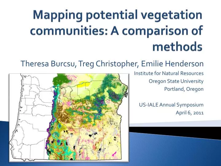
Mapping potential vegetation communities: A comparison of methods. Theresa Burcsu, Treg Christopher, Emilie Henderson Institute for Natural Resources Oregon State University Portland, Oregon US-IALE Annual Symposium April 6, 2011. Potential Vegetation Modeling/Mapping.

E N D
Mapping potential vegetation communities: A comparison of methods Theresa Burcsu, Treg Christopher, Emilie Henderson Institute for Natural Resources Oregon State University Portland, Oregon US-IALE Annual Symposium April 6, 2011
Potential Vegetation Modeling/Mapping • Plant Associations->PAGs->PVTs (VDDT)->Series/Veg Zone • Sources of uncertainties in maps • Field-based plot errors • Positional errors (GPS accuracy) • Misclassification of plant associations • Grouping plant associations • Quality of environmental inputs • Temp and precip from pts • DEM & derived variables • Modeling methods • Regression (NL) • Classification (RF and RFNN) • Assessment Methods • (FIA) plot validation • Map comparisons
PAG Method 1: Non-linear Regression • Methods • Estimation of lower bound for each PAG (Elev as depvarb) • Fitting a curve on each variable (or combo) to obtain coefficients for the regression equation • Displaying results on the landscape, field checking and re-fitting to match reality • Advantages: • An ecologist, with extensive local knowledge, can map a reasonably large area (NF District/L4 Ecoregion) with a high degree of accuracy • Consistent with ecological theory of potential -> defining lower limits not central tendency • Disadvantages: • Labor intensive • Because of the iterative nature of the method, regression equations are over-fit/calibrated -> not applicable to another location
PAG Method 2: (Classification Tree)->Random Forest (RF)->Random Forest w/ Imputation (RFNN) Elevation < 1244 August Maximum < 23.24 Temp August Maximum < 25.60 Temp LANDSAT Band 5 < 24 Summer Mean < 12.79 Temp Aug. to Dec. Temperature < 12.79 Differential Elevation < 1625 PSME PIPO TSHE PSME ABAM TSME PSME THPL High Elevation ( > 1244) High August Temp (> 23.24°C) High reflectance in Band 5 (> 24) Classification Tree is like a dichotomous key -rules created from plot data -used to key out each pixel
Random Forest (RF) A “Forest” of classification trees (default=1,000) Each tree is built from a random subset of plots and variables Rule set for each dichotomy varies from tree to tree Final call for a pixel is based on a majority vote PIPO PSME PIPO PSME PIPO PIPO
RF and RFNN Advantages • RF Advantages: • OK to include large # environmental inputs • No variable transformation needed • Robust to problem of collinearity • RFNN Advantages • Resistant to bias from unequal sample sizes between categories RF RFNN
Map Validation with Plots: The contingency table Reference PAG (FIA) • Kappa Statistic • Kappa measures the percentage agreement between one set of data (e.g. “truth”/plots) and another (model/maps), corrected for the amount of agreement that could be expected due to chance (i.e.“Error” or “Confusion” matrix) NL Model
Results: The contingency table • Other validation statistic to consider • Kappa per category • Tau • Area Under Curve Interpretation of agreement from Kappa .2 .4 .6 0 .8 1 Poor Fair Moderate Good Excellent
Map Comparison • How well do random forest models perform against a reference map? • Where are differences occurring? • Methods for comparison • Kappa • Fuzzy Kappa (KFuzzy) • Visual assessments 10
Kappa, the map version Kappa = KHisto * KLoc • KHisto • Similarity in quantity are the histograms similar? • KLoc • Similarity in location are the spatial distributions similar? • Cell-by-cell comparison Pontius 2000; Hagen 2002
Results: Kappa by PAG (NL vs RFNN) NLRFNN NLRFNN Moist Shasta red fir (ABMAS) NLRFNN (Western hemlock) Dry Shasta red fir; Mtn Hemlock
Fuzzy Kappa • Fuzzy location • Generates fuzzy membership matrix based on: • Neighborhood size • Distance decay function • Fuzzy categories • Similarities between categories • Fuzzy membership based on: • Ecological similarities between map classes • Derived from Bray-Curtis similarity index (species % cover) • Similarities range from 0 to 1 • Often used together Hagen 2003
Map ComparisonKappa and Kfuzzy (Location only) Crisp Fuzzy
Results: Sensitivity to Fuzzy Kappa Settings Kappa FLoc: Fuzzy Kappa, Location only Nhd, Halving Distance FCat: Fuzzy Kappa, Category and Location FCat: Fuzzy Kappa, Category only
Result: Visual assessment Reference RF map
Conclusions • Validation of models against independent plot dataset • Is reference map really more truthful than the Random Forest method? • Comparison of different model/maps to assess: • Which plant communities have high levels of disagreement • If not a global-level disagreement, then where are those disagreements occurring and why->aids in improving the next round of modeling • Issues/Areas for Improvements • Why does increasing the fuzzy neighborhood lower the kappa?! • Creating a similarity index on indicator species rather than using all species on plots • For comparison purposes, redo Random Forest modeling with more data rather than the limiting to environmental inputs used in NL regression
Results: Kappa and Fuzzy Kappa by PAG (NL vs RF)(Neighborhood=0)
RF RFNN