Examining the Relationship Between Two Variables

1. Examining the Relationship Between Two Variables (Bivariate Analyses)

2. What type of analysis? • We have two variables X and Y and we are interested in describing how a response (Y) is related to an explanatory variable (X). • What graphical displays do we use to show the relationship between X and Y ? • What statistical analyses do we use to summarize, describe, and make inferences about the relationship?

3. Type of Displays

4. Fit Y by X in JMP In the lower left corner of the Fit Y by X dialog box you will see this graphic which is the same as the more stylized version on the previous slide. Y Variable/Response Data Type X Variable/Predictor Data Type

5. Type of Displays

6. Type of Analyses

7. Fit Y by X in JMP Y nominal/ordinal Y continuous X continuous X nominal/ordinal

8. List of Variables id – ID # for infant & mother headcir – head circumference (in.) leng – length of infant (in.) weight – birthweight (lbs.) gest – gestational age (weeks) mage – mother’s age mnocig – mother’s cigarettes/day mheight – mother’s height (in.) mppwt – mother’s pre-pregnancy weight (lbs.) fage – father’s age fedyrs – father’s education (yrs.) fnocig – father’s cigarettes/day fheight – father’s height lowbwt – low birth weight indicator (1 = yes, 0 = no) mage35 – mother’s age over 35 ? (1 = yes, 0 = no) smoker – mother smoked during preg. (1 = yes, 0 = no) Smoker – mother’s smoking status (Smoker or Non-smoker) Low Birth Weight – birth weight (Low, Normal) Example: Low Birthweight Study(Note: This is not NC one) Continuous Nominal

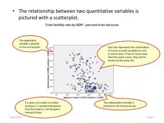
9. Example: Low Birthweight Study(Birthweight vs. Gestational Age) Y = birthweight (lbs.) Continuous X = gestational age (weeks)Continuous

10. Regression and Correlation Analysis from Fit Y by X

11. Example: Low Birthweight Study(Birthweight vs. Mother’s Smoking Status) Y = birthweight (lbs.) Continuous X = mother’s smoking status (Smoker vs. Non-smoker) Nominal

12. Independent Samples t-Test from Fit Y by X

13. Example: Low Birthweight Study(Birthweight Status vs. Mother’s Cigs/Day) Y = birthweight status(Low, Normal)Nominal X = mother’s cigs./day Continuous P(Low|Cigs/Day)

14. Logistic Regression from Fit Y by X

15. Example: Low Birthweight Study(Birthweight Status vs. Mother’s Smoking Status) Y = birthweight status(Low, Normal)Nominal X = mother’s smoking status (Smoker, Non-smoker)Nominal

16. Independent Samples p1 vs. p2 - Fisher’s Exact, Chi-square, Risk Difference, RR, & OR Skipped the arrows this time, everything should self-explanatory. Notice the OR is upside-down and needs reciprocation. OR = 1/.342 = 2.92

17. Summary In summary have seen how bivariate relationships work in JMP and in statistics in general. We know that the type of analysis that is appropriate depends entirely on the data type of the response (Y) and the explanatory variable or predictor (X).