Download
1 / 46
460 likes | 580 Views
Practice Final. John H. Vande Vate Spring 2006. Question 1. In class we described how a model that holds inventory of incoming supplies to buffer the supply chain from variations in customer demand. Question 1.

E N D
Practice Final John H. Vande Vate Spring 2006 1
Question 1 • In class we described how a model that holds inventory of incoming supplies to buffer the supply chain from variations in customer demand. 2
Question 1 • Under the model, the supplier normally ships the same quantity every day. When inventory rises to S, the model recommends curtailing shipments until it falls to Q and when inventory falls to 0, the model recommends expediting shipments or sending an unusually large shipment to bring inventory levels back up to q. 3
Question 1 Consider the special case in which: a. there is no inventory holding cost (h = 0) b. because of space limitations, the maximum inventory level S for the part cannot exceed a given level M c. the fixed costs of expediting and curtailing shipments are equal (K = L > 0) d. There are no variable costs for expediting and curtailing shipments (k = l = 0) 4
Question 1 What is the optimal strategy in this special case? S = Q = q = 5
Answer • S = M • Q = q = M/2 • Reasoning: Inventory is free, so we are only concerned with running into the bounds 0 and M, which we want to do as infrequently as possible. Since there are no variable costs to expedite and curtail, when we do expedite, we should expedite as much as we can to prevent having to expedite or curtail again. Symmetry leads us to Q = q = M/2 6
Question 2 • We argued in class that, under a periodic review regime, increasing the frequency of shipments generally reduces total inventory and expediting costs. We made this argument assuming that the costs of increasing frequency were negligible. 7
Question 2 • Suppose • inventory carrying costs are h = $100 per item per year • ordering costs are c = $1,000 per shipment • Demand over time is relatively constant at D = 200,000 per year • The average lead time is 4 weeks with a standard deviation of 2 days. • If we intend to hold safety stock constant regardless of the frequency of orders, how frequently should we order? 8
Solution • The lead time information is a red herring. It’s irrelevant as we have decided to hold safety stock constant. • This becomes a simple EOQ type problem with n, the number of times to order as the variable. The total cost formula is • hD/2n + cn • The solution is n = SQRT(hD/2c) = 100 9
Question 3 • We receive a shipment from our supplier once each week. The lead time for those shipments is 4 weeks with a standard deviation of 2 days. Demand each day is normally distributed with mean 100 and standard deviation 10. How much safety stock should we hold to ensure that the chances of stocking out before a shipment (not the annual chances of stocking out) are only 2%? 10
Solution • Calculate the variance in demand during the lead time plus the order period. This is (T+E[L])sD2 +D2sL2 • Careful with the units. Let’s work in days • T = 7 days • E[L] = 28 days • D = 100 units/day • sD2 = 100 units2/day • sL2 = 4 days2 11
Solution • So the variance is (T+E[L])sD2 +D2sL2 • 35*100+40,000 = 43,500 • And the standard deviation is about 208.5 units • We want to carry just over 2 standard deviations or about 417 items 12
Question 4 We ship products from Asia to Europe for sale to customers and are interested in strategies that reduce the “avoidable” costs of supply. • Under a periodic review regime, which of the following strategies will help reduce pipeline (in-transit) inventories? • Increasing frequency • Improving forecast accuracy • Reducing the safety lead-time • Moving our source for the products closer to Europe • Changing to a faster mode of transportation 13
Question 4 B. Under a periodic review regime, which of the following strategies will help reduce cycle inventories (on-hand inventory excluding safety stock)? • Increasing frequency • Improving forecast accuracy • Reducing the safety lead-time • Moving our source for the products closer to Europe • Changing to a faster mode of transportation 14
Question 4 C. Under a periodic review regime, which of the following strategies will allow us to reduce safety stock without compromising product availability? • Increasing frequency • Improving forecast accuracy • Reducing the safety lead-time • Moving our source for the products closer to Europe • Changing to a faster mode of transportation 15
Solution • Under a periodic review regime, which of the following strategies will help reduce pipeline (in-transit) inventories? • Increasing frequency • Improving forecast accuracy • Reducing the safety lead-time • Moving our source for the products closer to Europe • Changing to a faster mode of transportation 16
Question 4 B. Under a periodic review regime, which of the following strategies will help reduce cycle inventories (on-hand inventory excluding safety stock)? • Increasing frequency • Improving forecast accuracy • Reducing the safety lead-time • Moving our source for the products closer to Europe • Changing to a faster mode of transportation Only the first of these is direct. The rest are secondary effects achieved through improved forecast accuracy. We might argue that these only affected safety stock 17
Question 4 C. Under a periodic review regime, which of the following strategies will allow us to reduce safety stock without compromising product availability? • Increasing frequency • Improving forecast accuracy • Reducing the safety lead-time • Moving our source for the products closer to Europe • Changing to a faster mode of transportation We strongly suspect increasing frequency will reduce safety stock, but it is not always evident because we face the reduced risks more often. 18
Issues Raised in Projects • DaimlerChrysler Project • Which makes the most sense? • Front Suspension => Power Train => Assembly • Power Train => Front Suspension => Assembly • Power Train => Front Suspension => • The issues are: • Operating and Fixed Cost • Risk of shutting down assembly • Inventory • … Assembly 19
Risk of Shutting Down What is the issue? • Where do we want the bottleneck? • Important to note the relationships Front Suspension Power Train Power train Front Suspension Front Suspension Power Train Assembly Assembly Assembly Lost capacity at one process does NOT mean lost capacity at another 20
Joint Replenishment • Several parts from a single supplier • How often to ship and how much? • Assume every part on every truck • ci = unit cost of part I • Di = Annual demand for part I • N = number of joint shipments per year • T = cost of transportation per shipment • h = holding cost percentage • Total Cost = Ordering Costs + Inventory Costs 21
Joint Replenishment • Ordering Costs: T*N • N shipments at $T per shipment • Inventory Costs: • Di/N items per shipment • ciDi/N value of a shipment • hciDi/2N (one-sided inventory cost) • Total Cost • TN+sum (hciDi/2N) • N = sqrt(sum(hciDi/2)/T) • Qi = Di/N 22
Supply Consolidation • The replenishment is scheduled to share the transportation cost among products from the same supplier. • -Find the right demand Daily production x % Usage x Usage by BOM • Compute EOQ and T respectively for different parts • [step 1]:Round T to nearest power of two, minimal T* Re-compute order quantity (Q=DT) and thus holding cost with reduced transportation cost (A) • - [step 2]: Decrease T for all parts towards T* Re-compute order quantity (Q=DT) and thus holding cost with A unchanged 23
Team’s Approach • Don’t have every part on every truck • Compute EOQ quantities for each part to get Ti, the ideal time between shipments for each part • Take the smallest of these as T* • Trucks run that frequently • Other parts don’t get on every truck. Make them regular • Round Ti to one of 2T*, 4T*, 8T*… • I.e, gets on every other truck, every 4th truck, … • Step 2? 24
Newgistics Case • Economics • Pulling from RDU has three effects • Cost of pulling from RDU • Savings in postal costs to BMC • Reduced volume picked up from BMC and so (perhaps) truck costs • Hard part: • Estimate cost of pulling from RDU 25
Estimating RDU Costs • Carrier bags packages charges by bag based on weight • This charge is not $A/bag + $B/lb so… • This charge does include a fixed component per bag so…. Cost of Avg weight bag is not Avg cost of a bag The cost per package (inferred) rises as the volume at the RDU drops 26
The Optimization • What happens at 1 BMC has no impact on what happens at another – the problem separates • Variables: • How many trucks to the BMC • Whether of not to pull from each RDU • The objective is: • RDU pickup cost + • Postal cost to BMC + • Truck cost from BMW • Constraints are: • Enough trucks to meet frequency requirements at BMC • Enough trucks to meet volume requirements at BMC 27
Question • For you to think about: • How could you solve this problem if you did not have access to an optimization application? 28
BMW Projects • Frequency Project • Current Approach: Assumed transport costs across Atlantic are similar (turned out not true) • Optimize on the basis of lead-time • Simulate to determine • Total cost • Best split of shipments across routes • Interesting question: • Good model of total cost where variables are routes used and the quantities shipped on each 29
Ship-to-Average • Ship-to-Forecast • Places orders with regular frequency • But the order quantities change • Goal: Maintain regular inventory 30
Inventory • On-hand inventory* with ship-to-forecast: • constant level? *) Data of engine #7781905-00, high runner 31
Ship-to-Average • Increasing frequency • reduces relevant level of forecast accuracy • Increases shipment volatility 32
Use forecast accuracy over longer period of time! Use forecast accuracy over longer period of time! Use forecast accuracy over longer period of time! Forecast error • Why try to chase the daily forecast? % 33
Demand Variability* Standard Deviation: 42/day Mean Demand: 78/day *) Data of engine #7781905-00, high runner 34
Ship-to-Average • Reduces the variability in the order quantities • Does not raise the total avoidable cost • Simplifies the process 35
Goal #2 achieved! Shipment Comparison ship-to-forecast (shipment adjustment: 66%) = shipment quantity changes more than 10% compared to previous one ship-to-average (shipment adjustment: 14%) Shipment adjustments happen in 14% of all shipments 36
Part # 1092396-00 HIGH 6756673-00 HIGH 6762958-00 HIGH 7781905-00 HIGH 7783354-00 HIGH 1552166-00 LOW 6753862-00 LOW 7759119-00 LOW 7781903-00 LOW Total avoidable cost -0.36% -6.47% -5.70% -0.56% -0.45% -3.87% -1.67% -0.94% -3.85% Air cost +25.25% 77.14% +461.28% 57.71% -5.36% +15.22% 14.00% 60.45% 0.00% Shipment changes 47.11% 32.22% -16.32% 51.46% 55.83% 29.60% 48.84% 21.79% 56.04% Summary Table 37
Shelter First • Design a shelter and a logistics network to deliver it • Immediate (2-3 days) • Temporary • Change in thinking • Old thinking: Framework agreements with suppliers • Source from low cost countries • Often poorly served by international carriers 39
500 to 2000 miles ~ 100 miles Supplier Staging Area Warehouse Beneficiaries (Disaster Zone) Current Thinking Before Disaster • Supplier to Pre-positioned stock • $’s are driver. • Use ocean and ground After Disaster • Warehouses to Staging Area • Time is the driver • Use Commercial Air freight • Staging Area to Beneficiaries • If feasible, airdrop • If not, boats, helicopters, small trucks, animal carts… 40
Response Time Current Timeline Mobilization and Procurement (21 days) Delivery to Beneficiaries (7 days) Proposed Timeline Long Haul Transit (1-2 day) Last “100-Mile” (1-2 day) Mobilization (3 days) 41
Challenges • Limited space available on commercial aircraft on short-notice basis • Charters appear to offer potential solution • Design requirements of the shelter must be more focused on the goal • Immediate (smaller and lighter) • Temporary (so smaller and lighter may be ok) • Questions: Models to balance pre-positioned stocks vs expensive air freight in an environment of tight budgets and volatile demand. 42
Milliken Domestic and XYZ • Freight Consolidation • Where are the opportunities? • Volume • Sensitivity to distance • What are the economics? • Very hard to estimate LTL rates on lanes we don’t use • What Supply/Demand? • Model each customer/supplier or aggregate? • Volatility and Service • Model uses average volumes through consolidation, actual volumes fluctuate • Both a frequency and a volume component to truck costs • Optimization limitation (other) • Fooling the fixed costs 43
Milliken Asia • Model of total costs based on number and location of DCs • How is this different than BMW Frequency project? (Claim: It’s harder) • Data issues • Too much required, too little available • Demand! What other approaches? • Safety Stock: How to calculate from historical order information 44
Projects • I hope you have gotten meaningful feedback from me and your sponsor on your projects. If not. See me. • Pleased with level of work. Always possible to do more, better, … • Get me your files! Organized • Assessment of contributions (any form) • If you want to participate in Summer Special Topics Course get a Request for Approval of Special Projects form from Pam or Valarie for me to sign 45
Exam • Scheduled for 11:30 – 2:20 Friday May 5 • Flexible about dates • Can’t hurt your grade 46