Download

1 / 35
360 likes | 452 Views
CT image testing. What is a CT image?. CT= computed tomography Examines a person in “slices” Creates density-based images. Three different window densities. Bone- densest only bone shows detail, the rest is too dark to make out

E N D
What is a CT image? • CT= computed tomography • Examines a person in “slices” • Creates density-based images
Three different window densities • Bone- densest only bone shows detail, the rest is too dark to make out • Soft tissue- moderate density, bone is white, soft tissue is detailed, and “air space” is too dark • Lung- low density, bone and soft tissue white, and “air space” is detailed
How diagnoses are decided • Look for “abnormalities” in density
Our project- dare to compare • Test the new “unified LSU CT image”
Hypothesis • Unified LSU CT image: • Equally accurate • Faster
Methods • Our test • ROC Analysis • ROCKit Software
ROC Receiver Operating Characteristics Developed in 1950’s Statistical decision theory Used in business, economics, etc Goal: Is to be a meaningful tool for judging the performance of a diagnostic imaging system
Example • X Population y healthy z diseased • Gaussian distribution • Decision boundary • Interested in optimum decision boundary
EXAMPLE Non-diseased cases Diseased cases Threshold
EXAMPLE Non-diseased cases Diseased cases more typically:
DECISION BOUNDARY • TRUE NEGATIVE • TRUE POSITIVE • FALSE NEGATIVE • FALSE POSITIVE • What happens when you place the decision boundary?
DECISION BOUNDARY Non-diseased cases FALSE NEGATIVE IN RED Threshold Diseased cases TRUE POSITVE IN GREEN
DECISION BOUNDARY Non-diseased cases TRUE NEGATIVE IN WHITE Threshold Diseased cases FALSE POSITIVE IN WHITE
SENSITIVITY TPF Non-diseased cases SENSITIVITY = TP / TP + FN GREEN /GREEN+RED FNF = 1-TPF Threshold Diseased cases
SPECIFICITY TNF Non-diseased cases SPECIFICITY = TN / TN + FP LARGE WHITE / LARGE WHITE + SMALL WHITE FPF = 1-TNF Threshold Diseased cases
PREVALENCE • One of the important properties of ROC is that it is prevalence independent • Low prevalence is rare • Example • ROC IS NOT PREVALENCE DEPENDENT!
ROC CURVE Entire ROC curve TPF, sensitivity FPF, 1-specificity
ROC EXPERIMENT • Datasets • Two options • BINARY • MULT-SCALE RATING • Fitting curves
Rockit • Who developed Rockit? -Charles E. Metz @University of Chicago • What is Rockit? -curve fitting software calculates points for a Roc curve -calculates max probability of two Gaussian distributions • What is a Roc Curve? -describes how good the imaging systems is and accuracy of the given data and viewer’s results
Example 1 • 100 patients, 40 negative, 60 positive Given P P N P N N P… • Confidence Rating 1. Definitely Negative 2. Possibly Negative 3. Not sure 4. Possibly Positive 5. Definitely Positive This is the viewer’s results 5 4 2 4 1 2 3…. Now, from the confidence rating we consider 1=N and 2, 3, 4, 5=P to interpret view’s results. Interpretation of viewer’s result P P P P N P P… Comparing given data and interpretation TP TN FP FN 45 25 0 13 (a) TP- disease is present, diagnosed correctly (b) TN-disease is not present, diagnosed correctly (c) FP-person been diagnosed not having the disease, but the disease is present (d) FN-person been diagnosed having the disease, but the disease is not present. • Now, we compute the FPF and TPF. In order to compute the FPF, you need this formula FPF=1-TP/TP+FN and TPF=1-TN/TN+FP. • Therefore, in our case FPF=1-45/45+13= .224 and TPF=1-25/25+0=0 • So, our first point is (.224, 0).
Example 2 • Now we can compute a second point on the Roc curve. • We consider a different confidence rating. • 1, 2=N and 3, 4, 5=P Results based on viewer’s answer from above P P N P N N N N…. • The new Truth table is: TP TN FP FN 46 28 0 15 • Now the FPF=1-46 / 46+15 =.245 and TPF= 1-28/ 28+0 = 0 • Now, we have our second point (.245, 0) • Based upon the viewer’s results, a third and forth point can be created by changing the confidence ratings. 1, 2, 3=N and 4, 5=P ->third point 1, 2, 3, 4=N and 5=P ->forth point • Therefore, five confidence ratings give you four points on the Roc curve.
Rockit input • For Condition 1: d Enter the Total Number of Actually-Negative Cases (an integer): 40 Beginning with category 1 and separated by blanks, Enter (on one line, integers only) the number of responses to Actually- Negative cases in each category: 1 2 3 4 5 23 10 2 3 2 • For Condition 1: d Enter the Total Number of Actually-Positive Cases (an integer): 60 Beginning with category 1 and separated by blanks, Enter (on one line, integers only) the number of responses to Actually- Positive cases in each category: 1 2 3 4 5 2 2 3 10 43
Rockit • a, b parameters - a represents separation of the Gaussian distributions -b represents width of two Gaussian distributions • Open excel template to enter a, b parameters • Roc curve is produced