Download
1 / 40
400 likes | 660 Views
Sorting Algorithms. Sections 7.1 to 7.7. Comparison-Based Sorting. Input – 2,3,1,15,11,23,1 Output – 1,1,2,3,11,15,23 Class ‘ Animals ’ Sort Objects – Rabbit, Cat, Rat ?? Class must specify how to compare Objects In general, need the support of ‘<‘ and ‘>’ operators.

E N D
Sorting Algorithms Sections 7.1 to 7.7
Comparison-Based Sorting • Input – 2,3,1,15,11,23,1 • Output – 1,1,2,3,11,15,23 • Class ‘Animals’ • Sort Objects – Rabbit, Cat, Rat ?? • Class must specify how to compare Objects • In general, need the support of • ‘<‘ and ‘>’ operators
Sorting Definitions • In place sorting • Sorting of a data structure does not require any external data structure for storing the intermediate steps • External sorting • Sorting of records not present in memory • Stable sorting • If the same element is present multiple times, then they retain the original relative order of positions
C++ STL sorting algorithms • sortfunction template • void sort(iterator begin, iterator end) • void sort(iterator begin, iterator end, Comparator cmp) • begin and end are start and end marker of container (or a range of it) • Container needs to support random access such as vector • sort is not stable sorting • stable_sort() is stable
Heapsort Min heap Build a binary minHeap of N elements O(N) time Then perform NfindMin and deleteMinoperations log(N) time per deleteMin Total complexity O(N log N) It requires an extra array to store the results Max heap Storing deleted elements at the end avoid the need for an extra element 5
Example (MaxHeap) After BuildHeap After first deleteMax 7
Bubble Sort • Simple and uncomplicated • Compare neighboring elements • Swap if out of order • Two nested loops • O(n2)
Bubble Sort vector a contains n elements to be sorted. for (i=0; i<n-1; i++) { for (j=0; j<n-1-i; j++) if (a[j+1] < a[j]) { /* compare neighbors */ tmp = a[j]; /* swap a[j] and a[j+1] */ a[j] = a[j+1]; a[j+1] = tmp; } } http://www.ee.unb.ca/petersen/lib/java/bubblesort/
Bubble Sort Example 2, 3, 1, 15 2, 1, 3, 15 // after one loop 1, 2, 3, 15 // after second loop 1, 2, 3, 15 // after third loop
Insertion Sort • O(n2) sort • N-1 passes • After pass p all elements from 0 to p are sorted • Following step inserts the next element in correct position within the sorted part
Insertion Sort - Analysis • Pass p involves at most p comparisons • Total comparisons = ∑i ; i = [1, n-1] • = O(n²)
Insertion Sort - Analysis • Worst Case ? • Reverse sorted list • Max possible number of comparisons • O(n²) • Best Case ? • Sorted input • 1 comparison in each pass • O(n)
Lower Bound on ‘Simple’ Sorting • Simple sorting • Performing only adjacent exchanges • Such as bubble sort and insertion sort • Inversions • an ordered pair (i, j) such that i<j but a[i] > a[j] • 34,8,64,51,32,21 • (34,8), (34,32), (34,21), (64,51) … • Once an array has no inversions it is sorted • So sorting bounds depend on ‘average’ number of inversions performed
Theorem 1 • Average number of inversions in an array of N distinct elements is N(N-1)/4 • For any list L, consider reverse list Lr • L: 34, 8, 64, 51, 32, 21 • Lr: 21, 32, 51, 64, 8, 34 • All possible number of pairs is in L and Lr • = N(N-1)/2 • Average number of inversion in L = N(N-1)/4
Theorem 2 • Any algorithm that sorts by exchanging adjacent elements requires Ω(n²)average time • Average number of inversions = Ω(n2) • Number of swaps required = Ω(n2)
Bound for Comparison Based Sorting • O( n logn ) • Optimal bound for comparison-based sorting algorithms • Achieved by Quick Sort, Merge Sort, and Heap Sort
Mergesort Divide the N values to be sorted into two halves Recursively sort each half using Mergesort Base case N=1 no sorting required Merge the two (sorted) halves O(N) operation 20
Merging O(N) Time In each step, one element of C gets filled Each element takes constant time So, total time = O(N) 21
Mergesort Complexity Analysis Let T(N) be the complexity when size is N Recurrence relation T(1) = 1 T(N) = 2T(N/2) + N T(N) = 4T(N/4) + 2N T(N) = 8T(N/8) + 3N … T(N) = 2kT(N/2k) + k*N For k = logN T(N) = NT(1) + N logN Complexity: O(N logN) 25
Quicksort Fastest known sorting algorithm in practice Caveats: not stable Average case complexity O(N logN ) Worst-case complexity O(N2) Rarely happens, if implemented well http://www.cs.uwaterloo.ca/~bwbecker/sortingDemo/ http://www.cs.ubc.ca/~harrison/Java/ 26
Quicksort Outline Divide and conquer approach Given array S to be sorted If size of S < 1 then done; Pick any element v in S as the pivot PartitionS-{v} (remaining elements in S) into two groups S1 = {all elements in S-{v} that are smaller than v} S2 = {all elements in S-{v} that are larger than v} Return {quicksort(S1) followed by v followed by quicksort(S2) } Trick lies in handling the partitioning (step 3). Picking a good pivot Efficiently partitioning in-place 27
Quicksort Example 81 31 57 75 43 13 0 92 65 26 31 57 75 81 43 13 65 26 0 92 31 57 13 26 0 43 81 92 75 75 81 92 0 13 26 31 43 57 0 13 26 31 43 57 65 75 81 92 Select pivot partition 65 Recursive call Recursive call Merge 28
Quicksort Structure • What is the time complexity if the pivot is always the median? • Note: Partitioning can be performed in O(N) time • What is the worst case height 29
Picking the Pivot How would you pick one? Strategy 1: Pick the first element in S Works only if input is random What if input S is sorted, or even mostly sorted? All the remaining elements would go into either S1 or S2! Terrible performance! 30
Picking the Pivot (contd.) Strategy 2: Pick the pivot randomly Would usually work well, even for mostly sorted input Unless the random number generator is not quite random! Plus random number generation is an expensive operation 31
Picking the Pivot (contd.) Strategy 3: Median-of-threePartitioning Ideally, the pivot should be the median of input array S Median = element in the middle of the sorted sequence Would divide the input into two almost equal partitions Unfortunately, its hard to calculate median quickly, even though it can be done in O(N) time! So, find the approximate median Pivot = median of the left-most, right-most and center element of the array S Solves the problem of sorted input 32
Picking the Pivot (contd.) Example: Median-of-threePartitioning Let input S = {6, 1, 4, 9, 0, 3, 5, 2, 7, 8} left=0 and S[left] = 6 right=9 and S[right] = 8 center = (left+right)/2 = 4 and S[center] = 0 Pivot = Median of S[left], S[right], and S[center] = median of 6, 8, and 0 = S[left] = 6 33
Partitioning Algorithm Original input : S = {6, 1, 4, 9, 0, 3, 5, 2, 7, 8} Get the pivot out of the way by swapping it with the last element Have two ‘iterators’ – i and j i starts at first element and moves forward j starts at last element and moves backwards 8 1 4 9 0 3 5 2 7 6 pivot 8 1 4 9 0 3 5 2 7 6 i j pivot 34
Partitioning Algorithm (contd.) While (i < j) Move i to the right till we find a number greater than pivot Move j to the left till we find a number smaller than pivot If (i < j)swap(S[i], S[j]) (The effect is to push larger elements to the right and smaller elements to the left) Swap the pivot with S[i] 35
Partitioning Algorithm Illustrated i j pivot 8 1 4 9 0 3 5 2 7 6 i j Move pivot 8 1 4 9 0 3 5 2 7 6 i j pivot swap 2 1 4 9 0 3 5 8 7 6 i j pivot move 2 1 4 9 0 3 5 8 7 6 i j pivot swap 2 1 4 5 0 3 9 8 7 6 j i pivot i and j have crossed move 2 1 4 5 0 3 9 8 7 6 Swap S[i] with pivot 2 1 4 5 0 3 6 8 7 9 j i pivot 36
Dealing with small arrays For small arrays (say, N ≤ 20), Insertion sort is faster than quicksort Quicksort is recursive So it can spend a lot of time sorting small arrays Hybrid algorithm: Switch to using insertion sort when problem size is small (say for N < 20) 37
Quicksort Pivot Selection Routine Swap a[left], a[center] and a[right] in-place Pivot is in a[center] now Swap the pivot a[center] with a[right-1] 39
Quicksort routine Has a side effect move swap 40