Download
1 / 22
220 likes | 328 Views
Conditional distribution of the H-coefficient in nonparametric unfolding models. Andre Dabrowski Herold Dehling Wendy Post. Outline. Some aspects of unfolding models A conditional CLT Elements of the proof Remarks. Unfolding Models.

E N D
Conditional distribution of the H-coefficient in nonparametric unfolding models. Andre Dabrowski Herold Dehling Wendy Post
Outline • Some aspects of unfolding models • A conditional CLT • Elements of the proof • Remarks
Unfolding Models • Coombs(1964) introduced unfolding theory (parallelogram analysis) for dichotomous data in psychometrics • Each subject is asked to pick those stimuli he prefers from a list. • The goal is find an ordering (scale) or latent variable (ideal point) that would explain the preferences of subjects. • Item response theory, preference analysis, MDS
Unfolding Models • There is always someone I can talk to about my day to day problems • There are plenty of people I can lean on in case of trouble • There are many people I can count on completely • There are enough people that I feel close to • I can call on my friends whenever I need them • From DeJong Gierveld loneliness scale
Unfolding Models • We have m observations on N subjects Stimulus
Can we re-order the stimuli on a linear scale and define an ‘ideal’ point on that scale so that all stimuli within a fixed distance are chosen, and the rest are not? • Unfolding scale
Coombs’ model was deterministic and you can easily see that minor deviations in the data could render the problem insoluble. • E.g.
Several probabilistic models have been introduced to allow • P[subject picks stimulus k]=pk • Today we look at a model introduced by van Schuur (1984) and further developed by van Schuur and Post (1984). • MUDFOLD – a nonparametric method for Multiple UniDimensional unFOLDing
MUDFOLD • The data are assumed to be modelled by something between the deterministic Coombs model • And one where positive responses are placed at random given the marginal popularities of each stimulus.
Stimulus Allocate 1’s by sampling without replacement
Is (all or a part of) a list scalable or random? • Following Mokken (1971), van Schuur developed a coefficient of scalability based on Loevinger’s homogeneity coefficient. • H-coefficient for a given scale is defined by counting the number of ‘errors’ in choosing stimuli. • There is an error if the sequence of observations for a subject contains a 101 pattern.
For a single ordered triple ‘abc’ of stimuli in the order they appear in the unfolding scale, we count an error each time we observe a subject with the response ‘101’.
The score, M(s), for a single stimulus ‘s’ is the total number of errors over all triples containing ‘s’. • The ‘whole scale’ score, M, looks at the total over all possible ordered triples. • H(abc)=H(i)=1-M(i)/E*(M(i)) • H=1-M/E*(M)
Post (1989) obtained formulae for E(M) and Var(M) when unconditional popularities are known. • Post (1991) obtained formulae for E*(M) and Var*(M). • Now you can gauge the strength of scalability by H • Conditional CLT? Almost surely,
Expect normality as for contingency tables • Maejima (1970) established asymptotic normality for hypergeometric • There is work on conditional limits (Steck (1957), Holst (1981) • We decided to pursue an elementary proof based on the Laplace-deMoivre proof of the CLT, and Stirling’s formula.
For a single triple i=(i1, i2, i3) • Where for k=(k1, k2, …, km) in {0,1}m, • Nk is the count of subjects with Xji=ki and • K is the set of k where k(i1)=1, k(i2)=0 and k(i3)=1.
Following the classical proof, our approach will be to develop the conditional density of • {Nk, k in {0,1}m} given N1, N2, … Nm • And integrate to obtain a conditional CLT. • We then project to obtain the result for score triples. Lemma 1 Whenever
Lemma 2 Whenever x=(xk: k in {0,1}m) belongs to the lattice of points L={(zk-Npk)/N1/2: zk non-negative integers}.
Lemma 3 The discrete conditional density on L converges weakly to a normal density on the subspace L. Here L is a (2m-m-1)-dimensional subspace of and the normal density is given by These three lemmas prove the conditional CLT.
Projecting onto the subspace defined by score triples we obtain that the conditional joint distribution of score triples is asymptotically normal. Mean and covariances given in Post (1991). • Projecting onto the subspace defined by a single stimulus or the whole-scale H-coefficient, we obtain approximate normality for those statistics. Mean and covariances given in Post (1991). • Using a result of Steerneman (1986) on the rate of approximation of a hypergeometric by a normal, one can obtain a Berry-Esséen result for a single score triple.