Download
1 / 58
580 likes | 736 Views
Forecasting Space Weather with Dynamic Coronal Models. B.T. Welsch, W.P. Abbett, J. McTiernan, G.H. Fisher, Space Sciences Laboratory, University of California, Berkeley. Forecasting Space Weather with Dynamic Coronal Models. Why must we model the coronal field?

E N D
Forecasting Space Weather with Dynamic Coronal Models B.T. Welsch, W.P. Abbett, J. McTiernan, G.H. Fisher, Space Sciences Laboratory, University of California, Berkeley
Forecasting Space Weather with Dynamic Coronal Models • Why must we model the coronal field? • Why must our coronal models be dynamic? • What are the necessary components of a data-driven coronal model? • What is the current state of data-driven coronal modeling efforts? • What challenges remain?
Photospheric field evolution is often “boring.” Magnetograms of AR 8210 from MDI over ~24 hr. on 01 May 1998 show the field changing slowly. Proper motions are ~1 km/s.
Photospheric evolution is not dramatic; instead, it is slow, and seems steady.
Meanwhile, in the corona… … an M-class flare & halo CME occurred. CMEs can reach speeds of ~1000 km/s or more.
Differences between photospheric & coronal evolution led to the “storage & release” paradigm. • The coronal magnetic field is force-free (J x B = 0), but is “line-tied” to the photospheric field. • The photospheric field is not force-free (J x B0). • Photospheric flows (driven by, e.g., convection) slowly (v ~ 1 km/s) inject energy into the coronal field, which is stored in electric currents. • The high temperature and long length scales of the coronal plasma prevent dissipation of large scale currents (LvA/ ~ 1015). • Eventually, reconnection occurs, disspating / ejecting currents, and the coronal relaxes (at vA~103 km/s).
Free magnetic energy is the difference in energy between the actual and potential coronal fields. • For a given field B, the magnetic energy is U dV (B·B)/8. • The lowest energy the field could have would match the same boundary condition Bn, but would be current-free (curl-free), or “potential:” B(P) = - , with 2 = 0. U(P) dV (B(P) ·B(P) )/8 = dA ( n)/8 • The difference U(F) = U – U (P) is the energy available to power flares & CMEs!
One “storage & release” prediction: the coronal field should evolve toward the potential state. Pevtsov et al. (1996) saw this “sigmoid- to- arcade” evolution. Sigmoids are now widely viewed as signs of non-potentiality, and likelihood of eruption (Canfield et al., 1999).
How can photospheric magnetograms be used to forecast flares / CMEs? • Empirical Approach: With a high N sample, contrast flare / CME and “quiet” magnetograms. • H. Wang, previous talk! • Falconer et al. (2003, 2006) have used the length of the “strong gradient neutral line,” LSG in BLOS • good correlation with CMEs • “forecast window” t = +2 days • not normed by AR size, so: big ARs CMEs? • see poster by Yokoyama & Notoya re: strong gradients • Leka & Barnes (2003) found LSG had no significant correlation with flares on t = ~ 20 min.
Currently, short term forecasts from photospheric magnetograms alone are of limited utility. • For t ~ 1 hr., “no flare” is statistically the best bet – flares / CMEs are sporadic. • Many other possible models, however, have yet to be tested. Here are just a few… • Barnes et al. (2005): coronal “magnetic charge topology” • Wheatland & Metcalf (2005): magnetic virial theorem • Longcope & Magara (2004): “minimum current corona” • Welsch (2006): free energy flux
Aside: Flux emergence might trigger some eruptions, but is neither sufficient nor necessary for eruption. • Sometimes CMEs occur after emergence --- but only days later. (The coronal Alfvén crossing time is ~102 sec.) • Further, decayed active regions (showing no emergence) can erupt repeatedly. From “The Initiation of Coronal Mass Ejections by Newly Emerging Flux,” by J. Feynman and S. Martin, JGR, v. 100, p. 3355-3367 (1995).
From “Filament Eruptions near Emerging Bipoles,” Wang, Y.-M., and Sheeley, N. R., ApJ v. 510, p. L157: “It has been suggested in previous studies that quiescent prominences and filaments erupt preferentially in the vicinity of emerging magnetic flux. … Because eruptions sometimes occur in the absence of any observable flux emergence, however, we conclude that new flux may act as a strong catalyst but is not a necessary condition for filament destabilization.”
“Potentiality” should imply little free energy, and little likelihood of flaring. Schrijver et al. (2005) found potential ARs were not likely to flare.
“Non-potentiality” should imply non-zero free energy, and increased likelihood of flaring. Schrijver et al. (2005) found non-potential ARs were 2.4 times more likely to flare.
Forecasting Space Weather with Dynamic Coronal Models 1. Why must we model the coronal field? The coronal field drives flares / CMEs. 2. Why must our coronal models be dynamic? 3. What are the necessary components of a data-driven coronal model? 4. What is the current state of our data-driven coronal modeling efforts? 5. What challenges remain?
Forecasting Space Weather with Dynamic Coronal Models 1. Why must we model the coronal field? The coronal field drives flares / CMEs. 2. Why must our coronal models be dynamic? 3. What are the necessary components of a data-driven coronal model? 4. What is the current state of our data-driven coronal modeling efforts? 5. What challenges remain?
Potential NLFFF MHD Photosphere Chromosphere In some cases, non- linear force- free field (NLFFF) ex-trapolation can accurately reproduce a model coronal field. Abbett et al., JASTP (2004). Extrapolation from the chromospheric magnetic field (more force-free) is better, but chromospheric vector magnetograms are rare.
However, static extrapolations from a forced boundary cannot always reproduce a given magnetic field. An extrapolated non-linear force-free field’s energy can be far less than the energy in an MHD field, since it has evolved ~ideally. From Antiochos, DeVore, and Klimchuk, ApJ, v. 510, p. 485 (1999)
Forecasting Space Weather with Dynamic Coronal Models 1. Why must we model the coronal field? The coronal field drives flares / CMEs. • Why must our coronal models be dynamic? Static models can miss free magnetic energy. 3. What are the necessary components of a data-driven coronal model? 4. What is the current state of our data-driven coronal modeling efforts? 5. What challenges remain?
Aside: Vector magnetograms from a force- free layer should accurately reflect the state of the coronal field. • Since the photosphere is not force- free, it does not reflect the state of the coronal field. • The magnetic field is force- free in the upper chromosphere and above. • Extrapolations from a force- free layer (or applications of the magnetic virial theorem [Metcalf et al. 2002]) could be used as forecast tools. • Chromospheric vector magnetograms are rare!
Forecasting Space Weather with Dynamic Coronal Models 1. Why must we model the coronal field? The coronal field drives flares / CMEs. • Why must our coronal models be dynamic? Static models can miss free magnetic energy. 3. What are the necessary components of a data-driven coronal model? 4. What is the current state of our data-driven coronal modeling efforts? • What challenges remain?
How can time sequences of vector magneto-grams be used in dynamic coronal models? • Need a realistic initial condition. • Time dependent boundary condition necessary. • Realistic model of photosphere and corona. Hinode/FPP, SDO/HMI, and SOLIS/VSM can provide these data.
Aside: A “useful” data stream of magnetograms is essential for data driving, and entails: • Vector magnetograms; LOS won’t do. • Departures from potentiality in BHORIZ must be observationally determined. • A high “duty cycle” magnetograph, for adequate temporal coverage. • Practically, space-borne magnetographs are best. • Low cadence is prob’ly okay • v ~ 1 km/s 10 min. for x ~ 1 arc. sec.
Forecasting Space Weather with Dynamic Coronal Models 1. Why must we model the coronal field? The coronal field drives flares / CMEs. 2. Why must our coronal models be dynamic? Static models can miss free magnetic energy. • What are the necessary components of a data-driven coronal model? A useful data stream. 4. What is the current state of our data-driven coronal modeling efforts? 5. What challenges remain?
A realistic initial field must be determined. • Potential fields have no free energy, and therefore are not a good initial condition. • Non-linear force-free fields (NLFFFs) are the simplest realistic starting point. • Driven MHD relaxation can also be used, but is more time consuming. • We use the “optimization” method to determine an NLFFF initial condition (tested by Schrijver et al. 2006).
Here are some field lines for a potential field model for the first vector magnetogram in the AR 8210 sequence. The potential field was found using a Fourier method (Alissandrakis, 1981; Gary, 1989). Boundaries are periodic, but a guard ring of 0’s is put around the original magnetogram. For the energy calculation, a volume of 210x166x166 was used. Grid spacing is constant, 1.1 arcsec or 800 km. Slide courtesy J. McTiernan
Here are field lines, drawn from the same start points, for the NLFFF extrapolation. They do not look much different, except that the loops are higher, and there are a couple of sheared lines, at lower levels. The ‘start points’ are the left hand footpoint of each field line. Slide courtesy J. McTiernan
Forecasting Space Weather with Dynamic Coronal Models 1. Why must we model the coronal field? The coronal field drives flares / CMEs. 2. Why must our coronal models be dynamic? Static models can miss free magnetic energy. • What are the necessary components of a data-driven coronal model? A useful data stream; realistic initial condition. 4. What is the current state of our data-driven coronal modeling efforts? 5. What challenges remain?
The bottom boundary must be driven to match the observed B(x,y,z; t), from the magnetograms. Two techniques have been applied: • Method of Characteristics (MOC) Nakagawa (1980), Wu et al. (2001), Hayashi (2005) • Imposed velocity, v(x,y,0;t) equivalent to imposing electric field, E = - (v x B)/c
Either method of driving determines one of the MHD equations on the boundary. • MOC incorporates B/t directly, so the induction equation is not solved. • Imposing v(x,y,0;t) determines v/t, so the momentum equation is not solved.
Several techniques exist to determine velocities required to drive coronal magnetic field simulations. • Inductive Method (Kusano et al. 2000, 2005) • FLCT, ILCT (Welsch et al. 2004), • MEF (Longcope 2004), • DAVE (Schuck, 2006) • LCT (e.g., Démoulin & Berger 2003) • MSR (Georgoulis & LaBonte 2006). These flows can also be used to study the fluxes of magnetic energy and helicity into the corona.
Fourier local correlation tracking (FLCT) finds v(x1,x2) by correlating subregions. = * = = 4) v(xi, yi) is inter- polated max. of correlation funct 1) for ea. (xi, yi) above |B|threshold… 2) apply Gaussian mask at (xi, yi) … 3) truncate and cross-correlate…
Demoulin & Berger (2003) argued that LCT flows in magnetograms are not identical to plasma velocities. The apparent motion of flux on the photosphere, uf, is a combination of horizontal flows and vertical flows acting on non-vertical fields. uf vnBh-vhBn is the flux transport velocity • uf is the apparent velocity (2 components) • v is the actual plasma velocity (3 comps)
The ideal induction equation’s normal component relates velocities to dBn/dt. Bn/t = h(vnBh-vhBn) = -h(ufBn) • -h(uLCTBn) approximates Bn/t, so we assume uLCT uf • Inductive LCT (ILCT) finds uf that matches Bn/t exactly and closely matches uLCT. • Writing ufBn = -h + h x( n), we find • via Bn/t = h2 • by assuming uf = uLCT, so h2 = - h x(uLCTBn)
Tests with MHD simulations show that ILCT reproduces velocities better than FLCT does. Images from Welsch et al., in prep.
Driving the model to match the observed tangential field evolution requires specifying vertical derivatives of v(x1,x2). Initially from NLFFF extrapolation Directly measured Derived by ILCT Calculated by boundary code at photosphere, z = 0 above photosphere, z > 0
Forecasting Space Weather with Dynamic Coronal Models 1. Why must we model the coronal field? The coronal field drives flares / CMEs. 2. Why must our coronal models be dynamic? Static models can miss free magnetic energy. • What are the necessary components of a data-driven coronal model? A useful data stream; realistic initial condition, driving. 4. What is the current state of our data-driven coronal modeling efforts? 5. What challenges remain?
Mainly, a realistic model coupling the photosphere to the corona is needed. Several challenges exist: • Density decreases by ~10 orders of magnitude. • Temperature increases by ~2.5 orders of magnitude. • The photosphere-corona system is “stiff:” vA goes from 1 km/s 1000 km/s. • Photosphere is sub-sonic, but shocks are common in the chromosphere and corona. • Active region length scales are ~100 Mm, but current sheets can be less than 100 km.
W.P. Abbett’s code, RADMHD, is semi-implicit, Cartesian, parallel, and adaptively refined. (A manuscript is in prep.) Either an ideal equation of state, with = 5/3, or the non-ideal OPAL equation of state can be used. This code was specifically developed to enable realistic coupling of the photosphere to the corona.
The practical computational challenges were surmounted with a variety of techniques. • The MHD system is solved semi-implicitly on a block adaptive mesh. • The non-linear portion of the system is treated explicitly using the semi-discrete central method of Kurganov-Levy (2000) using a 3rd-order CWENO polynomial reconstruction • Provides an efficient shock capture scheme, AMR is not required to resolve shocks • The implicit portion of the system, the contributions of the energy source terms, and the resistive and viscous contributions to the induction and momentum equations respectively, is solved via a “Jacobian-free” Newton-Krylov technique • Makes it possible to treat the system implicitly (thereby providing a means to deal with temporal disparities) without prohibitive memory constraints 11
RADMHD’s treatment of the energy equation is sophisticated. • In the transition region and corona, optically thin radiative losses are assumed, QR -nenh(T) • Coronal heating QB|B| is assumed, after Pevtsov et al., 2003. • Anisotropic thermal conduction is scaled, after Mikic et al. (2005), to handle the transition region’s thin scale height (~ 1 km!) • Surface radiation is parameterized, and calibrated against more realistic simulations (e.g., Stein, Bercik & Nordlund, 2003) • Denser / lower layers include optically thick radiative diffusion, and can therefore convect.
Top row: Vertical momentum along horizontal slices at different depths in the 30x30x7.5 Mm3 domain. From left to right: ~1Mm below the visible surface, the photosphere, the upper chromosphere, and the low corona. Bottom row: the vertical component of the magnetic field along the same horizontal slices. The second and third frames can be thought of as a simulated LOS magnetogram at disk center --- note the difference between the photospheric and chromospheric magnetogram in the simulated Quiet Sun.
RADMHD can match the observed photosphere- to- corona density and temperature stratification.
Data Driving --- The Strategy: Model Corona “Active” Boundary Layer Observational Data / Flows 15
Forecasting Space Weather with Dynamic Coronal Models 1. Why must we model the coronal field? The coronal field drives flares / CMEs. 2. Why must our coronal models be dynamic? Static models can miss free magnetic energy. • What are the necessary components of a data-driven coronal model? A useful data stream; realistic initial condition, driving, and model. 4. What is the current state of our data-driven coronal modeling efforts? 5. What challenges remain?
Forecasting Space Weather with Dynamic Coronal Models 1. Why must we model the coronal field? The coronal field drives flares / CMEs. 2. Why must our coronal models be dynamic? Static models can miss free magnetic energy. 3. What are the necessary components of a data-driven coronal model? A useful data stream; realistic initial condition, driving, and model. 4. What is the current state of our data-driven coronal modeling efforts? 5. What challenges remain?
MPI-AMR relaxation test runs on active region scales are now underway. • Near-term tests: • Dynamically and energetically relax a 30Mm square Cartesian domain extending to ~2.5Mm below the surface. • Introduce a highly-twisted AR-scale magnetic flux rope (from the top of a sub-surface calculation) through the bottom boundary of the domain • Reproduce (hopefully!) a highly sheared, δ-spot type AR at the surface, and follow the evolution of the model corona as AR flux emerges into, reconnects and reconfigures coronal fields • The long term plan: • global scales / spherical geometery Q: How do different treatments of the coefficient of resistivity, or changes in resolution affect the topological evolution of the corona? 13
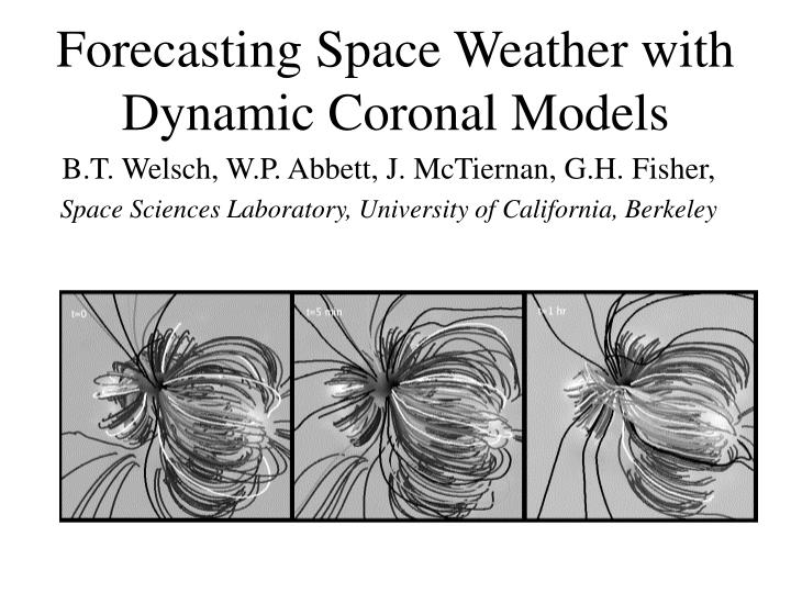
Although still being validated, we have run the code on active region data, to ensure it won’t crash! These images show relaxation of the initial atmosphere in AR 8210, on 01 May 1998.