Download
1 / 19
200 likes | 323 Views
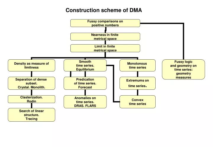
Construction scheme of DMA. DRAS global level. DRAS,FLARS, FCARS local level. FTS. Rectification of FTS. FLARS global level. FTS Anomalies. FCARS global level. FTS anomaly recognition algorithms: DRAS, FLARS and FCARS. DRAS (Difference Recognition Algorithm for Signals ) - 2003

E N D
DRASglobal level DRAS,FLARS,FCARS locallevel FTS Rectificationof FTS FLARSglobal level FTSAnomalies FCARSglobal level FTS anomaly recognition algorithms: DRAS, FLARS and FCARS • DRAS(Difference Recognition Algorithm for Signals ) - 2003 • FLARS(FuzzyLogic Algorithm for Recognition of Signals) – 2005 • FCARS (Fuzzy Comparison Algorithm for Recognition of Signals) - 2007 • realize “smooth” modeling (in fuzzy mathematics sense introduced by L. Zade) of interpreter’s logic, that searches for anomalies on FTS. Examples of FTS rectification functionals Length of the fragment, energy of the fragment, difference of the fragment from its regression of order n.
Interpreter’s Logic. Illustration Record Local level - rectificationofthe record Global level - searching the uplifts on rectification
DRAS and FLARS: local level - rectification Discrete positive semiaxes h+={kh; k=1,2,3,…} Record y={yk=y(kh), k=1,2,3,…} Registration period Y h+ Parameter of local observation Δ=lh, l=1,2,… Fragment of local observation Δky={yk-Δ/h ,… , yk ,… , yk+Δ/h}Δh+1 Definition. A non-negative mapping defined on the set of fragments {Δky}2Δ/h+1 we call by a rectifying functional of the given record “y”. We call any function ykΔky by rectification of the record “y”.
Examples of rectifications 1 Length of the fragment: 2 Energy of the fragment: 3 Difference of the fragment from its regression of order n: here as usual is an optimal mean squares approximation of order n of the fragment . If n=0 we get the previous functional “energy of the fragment”: 4 Oscillation of the fragment:
Illustration of rectification Record Rectification «Energy» Rectification «Length»
DRAS: Difference Recognition Algorithm for Signals. Left and Right background measures Potential anomaly on the record Record rectification Genuine anomaly on the record Record fragmentation Record Paris, 3-5 November 2004
DRAS: global level. Recognition of potential anomalies. - vertical level of background Left and right background measures of silence - β– horizontal level of background Potentialanomaly on the record y: PA={khY : min((LαΦy)(k), (RαΦy)(k)) < β} Regular behavior of the record y: B={khY : min((LαΦy)(k), (RαΦy)(k)) β}
DRAS: global level. Recognition of genuine anomalies. Potential anomalies PA = UP(i), n=1,2, N. is a union of coherent components DRAS recognizes genuine anomalies A(n) as parts of P(n) by analyzing operator DΦ(k) = LΦ(k) - RΦ(k). The beginning of A(n) is the first positive maximum of DΦ(k) on P(n). Indeed , the difference between “calmness” from the left and anomaly behavior from the right is the biggest in this point. By the same reason, the end of A(n) is in the last negative minimum of DΦ(k).
DRAS: recognition of genuine anomaly. Genuine anomalies on the record y, A = {alternating-sign decreasing segments for (DαΦy)(k)}
FLARS: Global level. recognition ofgenuine anomaly. α[0,1] – vertical level of how extreme are the measure values Genuine anomaly on the record yA = { kh Y : μ(k)α} Regular behavior/ potential anomalyNA = { kh Y : μ(k)<α}
FLARS: global level. Recognition of potential anomaly. We introduce the function that possesses the following properties: One-sided background measures - Θ – the parameter of intermediate observation: Δ<Θ≤Δ . β– horizontal level of background, (-1,1) Potentialanomaly on the record y PA={kh NA: min((LαΦy)(k), (RαΦy)(k)) < β} Regular behavior of the recordy B={kh NA: min((LαΦy)(k), (RαΦy)(k)) β}
FLARS: anomaly measure μ(k) - parameter of global observation δkk - model of global observation record at the point k The following sum will be an “argument” for minimality (regularity) of the point “kh” The following sum will be an “argument” for maximality (anomaly) of the point “kh” The measure is a result of the comparison of the “arguments” and
FLARS: recognition of anomaly on the record. Record Rectification Anomality measure
FLARS: application to the Superconducting Gravimeters data preprocessing(Strasbourg, France)
DRAS and FLARS recognition comparison DRAS FLARS
What algorithm to apply to FTS data sets? • DRAS. Calm and anomaly points are quite well distinguished, but genuine anomalies are not evident. DRAS is useful in searching big anomalies. • FLARS. High amplitude anomalies are quite obvious and small anomalies are not so evident on the background of noise. Useful to search very small isolated anomalies. • FCARS. Important in searching oscillating anomalies and identification of the beginning and ends of the signals.