Download
1 / 55
570 likes | 748 Views
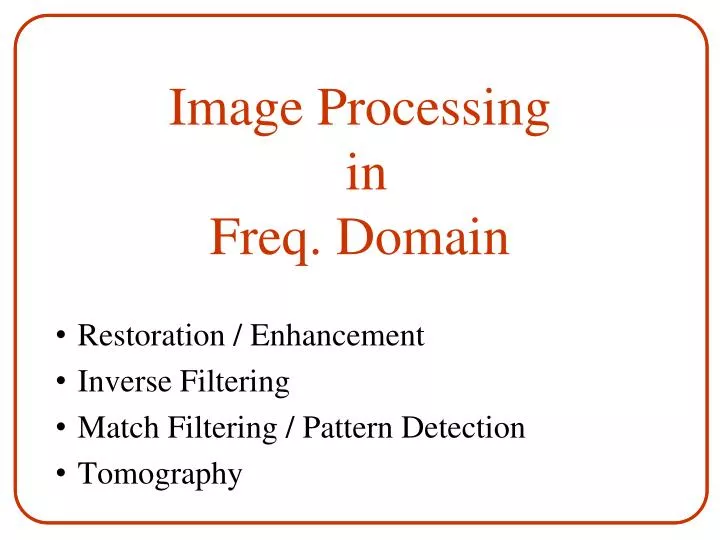
Image Processing in Freq. Domain . Restoration / Enhancement Inverse Filtering Match Filtering / P attern D etection Tomography. Enhancement v.s. Restoration. Image Enhancement : A process which aims to improve bad images so they will “ look ” better. Image Restoration :

E N D
Image Processing in Freq. Domain • Restoration / Enhancement • Inverse Filtering • Match Filtering / Pattern Detection • Tomography
Enhancement v.s. Restoration • Image Enhancement: • A process which aims to improve bad images so they will “look” better. • Image Restoration: • A process which aims to invert known degradation operations applied to images.
Enhancement vs. Restoration • “Better” visual representation • Subjective • No quantitative measures • Remove effects of sensing environment • Objective • Mathematical, model dependent quantitative measures
Typical Degradation Sources Low Illumination Optical distortions (geometric, blurring) Sensor distortion (quantization, sampling, sensor noise, spectral sensitivity, de-mosaicing) Atmospheric attenuation (haze, turbulence, …)
Image Preprocessing Restoration Enhancement • Denoising • Inverse filtering • Wiener filtering Freq. Domain Spatial Domain Filtering Point operations Spatial operations
Examples Hazing
Echo image Motion Blur
Blurred image Blurred image + additive white noise
Reconstruction Algorithm Reconstruction as an Inverse Problem noise Original image Distortion H measurements
So what is the problem? • Typically: • The distortion H is singular or ill-posed. • The noise n is unknown, only its statistical properties can be learnt.
Key point: Stat. Prior of Natural Images likelihood prior MAP estimation:
Most probable solution Bayesian Reconstruction (MAP) • From amongst all possible solutions, choose the one that maximizes the a-posteriori probability: P(f | g)P(g | f) P(f) P(f) measurements P(g|f) Image space
Bayesian Denoising • Assume an additive noise model : g=f + n • A MAP estimate for the original f: • Using Bayes rule and taking the log likelihood :
Bayesian Denoising • If noise component is white Gaussian distributed: g=f + n wheren is distributed ~N(0,) R(f) is a penalty for non probable f prior term data term
Inverse Filtering • Degradation model: g(x,y) = h(x,y)*f(x,y) G(u,v)=H(u,v)F(u,v) F(u,v)=G(u,v)/H(u,v)
Inverse Filtering (Cont.) Two problems with the above formulation: • H(u,v) might be zero for some (u,v). • In the presence of noise the noise might be amplified: F(u,v)=G(u,v)/H(u,v) + N(u,v)/H(u,v) Solution: Use prior information prior term data term
Option 1: Prior Term • Use penalty term that restrains high F values: where • Solution:
F=G/H
The inverse filter is C(H)= H*/(H*H+ ) • At some range of (u,v): S(u,v)/N(u,v) < 1 noise amplification. =10-3
Option 2: Prior Term • Natural images tend to have low energy at high frequencies • White noise tend to have constant energy along freq. where
Solution: • This solution is known as the Wienner Filter • Here we assume N(u,v) is constant. • If N(u,v) is not constant:
Wienner Previous
Matched Filter in Freq. Domain • Pattern Matching: • Finding occurrences of a particular pattern in an image. • Pattern: • Typically a 2D image fragment. • Much smaller than the image.
Image Similarity Measures • Image Similarity Measure: • A function that assigns a nonnegative real value to two given images. • Small measure high similarity • Preferable to be a metric distance (non-negative, identity, symmetric, triangular inequality) • Can be combined with thresholding: d( - ) ≥ 0
The Matching Approach • Scan the entire image pixel by pixel. • For each pixel, evaluate the similarity between its local neighborhood and the pattern.
The Euclidean Distance as a Similarity Measure • Given: • k×k pattern P • n×n image I • kxk window of image I located at x,y - Ix,y • For each pixel (x,y), we compute the distance: • Complexity O(n2k2)
Fixed FFT Implementation • Convolution can be applied rapidly using FFT. • Complexity: O(n2 log n)
Naïve vs. FFT Performance table for a 1024×1024 image, on a 1.8 GHz PC:
Normalized Cross Correlation • NCC: • A similarity measure, based on a normalized cross-correlation function. • Maps two given images to [0,1] (absolute value). • Measures the angle between vectors Ix,y and P • Invariant to intensity scale and offset.
Efficient Implementation • Note that • Thus, • The above expression can be implemented efficiently using 3 convolutions.
NCC similarity measure Euclidean distance similarity measure
Euclidean distance similarity measure NCC similarity measure
CT Scanners • In 1901 W.C. Roentgen won the Nobel Prize (1st in physics) for his discovery of X-rays. Wilhelm Conrad Röntgen
CT Scanners • In 1979 G. Hounsfield & A. Cormack, won the Nobel Prize for developing the computer tomography. • The invention revolutionized medical imaging. Allan M. Cormack Godfrey N. Hounsfield
Tomography: Reconstruction from Projection 1 f(x,y) 2
Projection & Sinogram • Projection: All ray-sums in a direction • Sinogram: collects all projections y P(t) t p x f(x,y) t X-rays Sinogram
CT Image & Its Sinogram K. Thomenius & B. Roysam
The Slice Theorem Fourier Transform y v 1 1 x u f(x,y) spatial domain frequency domain