Download
1 / 10
100 likes | 197 Views
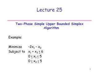
CS 547: Lecture 25. Continuous-time Markov Chains Mary K. Vernon Fall 2003. Today’s Outline. Formal definition of CTMCs Transient solution: P[X(t)=k] Steady state solution Applications M/M/1 queue Machine repair model Reference: AA 4.3, 5.0-5.2; LK1 2.4, 3.1.

E N D
CS 547: Lecture 25 Continuous-time Markov Chains Mary K. Vernon Fall 2003
Today’s Outline • Formal definition of CTMCs • Transient solution: P[X(t)=k] • Steady state solution • Applications • M/M/1 queue • Machine repair model Reference: AA 4.3, 5.0-5.2; LK1 2.4, 3.1
Continuous Time Markov Chains Definition: a stochastic process {X(t), tT} is a Markov process if t1,t2,…,tn+1, t1 t2 … tn+1 and x1,x1,…, xn+1, P[X(tn+1)xn+1 | X(t1)x1,X(t2)x2, …, X(tn)xn] P[X(tn+1)xn+1 | X(tn)xn] Continuous-timeMarkov chain (CTMC): state space is discrete, T is continuous e.g., Poisson counting process, or Q(t) in M/M/1 queue Goal: derive Pk(t) P[X(t) j] and/or j P[X(t) = j] Notation: pi,,j (t1,t2) = P[X(t2)j| X(t1)i]
0 1 2 3 CTMC: Graphical Representation state transition rates: , i j time-homogeneous: qi,j qi,j(t) pi,,j(t,t+h) qi,jh + o(h), i j pi,i(t,t+h) 1 ( qi,j)h + o(h) e.g.,X(t) is the queue length of an M/M/1 queue at time t qi,i+1 qi,i-1 State transitions are labelled with the state transition rate
CTMC: Pk(t) pi,j(t1,t2) P[X(t2)j| X(t1) i] P(t) P[X(t) j] theorem of total probability where Qi,i qi,j , i.e., pi,,i(t,t+h) 1 + qi,ih + o(h) Qi,j qi,j , ij
CTMC: Pk(t) pi,j(t1,t2) P[X(t2)j| X(t1) i] P(t) P[X(t) j] st or thus, and completely define a time-homogeneous CTMC
0 1 2 3 CTMC Example: Pk(t) X(t) = queue length of M/M/1 queue at time t , k 1 solution for Pk(t): LK1 pp. 74-77 (very complex)
0 1 2 2 CTMC Example: Pk(t) X(t) = number of machines that are operational at time t Solution for P0(t): AA Example 4.3.3, pp. 217-219
CTMC: P[X(t) = j] This “equilibrium distribution” or “stationary distribution” exists and is independent of the initial state if the DPMC is irreducible is non-trivial if the CTMC is irreducible & recurrent non-null in this case, and
0 1 2 3 k k U/(1 U) CTMC Example: k X(t) = queue length of M/M/1 queue at time t irreducible 0 - flux out of state k + flux into state k 0 -0 + 1 ; 0 -( + )1 + 0 + 2 ; 1 (/) 0 ; 2 (/)1 (/)2 0; … k (/)k 0 : 0[ 1 + (/)k ] 0 Uk 1 0 [ 1 U]1 1, or U 1 0 1 U, k (1 U)Uk E[Q] =