Download
1 / 32
320 likes | 445 Views
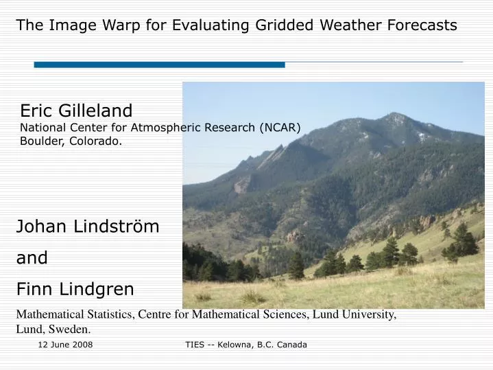
The Image Warp for Evaluating Gridded Weather Forecasts. Eric Gilleland National Center for Atmospheric Research (NCAR) Boulder, Colorado. Johan Lindström and Finn Lindgren Mathematical Statistics, Centre for Mathematical Sciences, Lund University, Lund, Sweden. F. O.

E N D
The Image Warp for Evaluating Gridded Weather Forecasts Eric Gilleland National Center for Atmospheric Research (NCAR) Boulder, Colorado. Johan Lindström and Finn Lindgren Mathematical Statistics, Centre for Mathematical Sciences, Lund University, Lund, Sweden. TIES -- Kelowna, B.C. Canada
F O User-relevant verification: Good forecast or Bad forecast? TIES -- Kelowna, B.C. Canada
F O User-relevant verification: Good forecast or Bad forecast? If I’m a water manager for this watershed, it’s a pretty bad forecast… TIES -- Kelowna, B.C. Canada
F O A B Flight Route User-relevant verification: Good forecast or Bad forecast? O If I’m an aviation traffic strategic planner… It might be a pretty good forecast Different users have different ideas about what makes a good forecast TIES -- Kelowna, B.C. Canada
Which rain forecast is better? Mesoscale model (5 km) 21 Mar 2004 Global model (100 km) 21 Mar 2004 Observed 24h rain Sydney Sydney RMS=13.0 RMS=4.6 High vs. low resolution From E. Ebert TIES -- Kelowna, B.C. Canada
Which rain forecast is better? Mesoscale model (5 km) 21 Mar 2004 Global model (100 km) 21 Mar 2004 Observed 24h rain Sydney Sydney RMS=13.0 RMS=4.6 High vs. low resolution “Smooth” forecasts generally “Win” according to traditional verification approaches. From E. Ebert TIES -- Kelowna, B.C. Canada
Traditional “Measures”-based approaches Consider forecasts and observations of some dichotomous field on a grid: Some problems with this approach: (1) Non-diagnostic – doesn’t tell us what was wrong with the forecast – or what was right (2) Ultra-sensitive to small errors in simulation of localized phenomena CSI = 0 for first 4; CSI > 0 for the 5th TIES -- Kelowna, B.C. Canada
Spatial forecasts Spatial verification techniques aim to: • account for uncertainties in timing and location • account for field spatial structure • provide information on error in physical terms • provide information that is • diagnostic • meaningful to forecast users Weather variables defined over spatial domains have coherent structureand features TIES -- Kelowna, B.C. Canada
Recent research on spatial verification methods • Filter Methods • Neighborhood verification methods • Scale decomposition methods • Motion Methods • Feature-based methods • Image deformation • Other • Cluster Analysis • Variograms • Binary image metrics • Etc… TIES -- Kelowna, B.C. Canada
Filter Methods Neighborhood verification • Also called “fuzzy” verification • Upscaling • put observations and/or forecast on coarser grid • calculate traditional metrics Ebert (2007; Met Applications) provides a review and synthesis of these approaches Fractions skill score (Roberts 2005; Roberts and Lean 2007) TIES -- Kelowna, B.C. Canada
Filter Methods Single-band pass • Errors at different scales of a single-band spatial filter (Fourier, wavelets,…) • Briggs and Levine, 1997 • Casati et al., 2004 • Removes noise • Examine how different scales contribute to traditional scores • Does forecast power spectra match the observed power spectra? Fig. from Briggs and Levine, 1997 TIES -- Kelowna, B.C. Canada
Feature-based verification Error components • displacement • volume • pattern TIES -- Kelowna, B.C. Canada
Numerous features-based methods Motion MethodsFeature- or object-based verification • Composite approach (Nachamkin, 2004) • Contiguous rain area approach (CRA; Ebert and McBride, 2000; Gallus and others) Gratuitous photo from Boulder open space TIES -- Kelowna, B.C. Canada
Motion MethodsFeature- or object-based verification • Baldwin object-based approach • Method for Object-based Diagnostic Evaluation (MODE) • Others… TIES -- Kelowna, B.C. Canada
Inter-Comparison Project (ICP) • References • Background • Test cases • Software • Initial Results http://www.ral.ucar.edu/projects/icp/ TIES -- Kelowna, B.C. Canada
The image warp TIES -- Kelowna, B.C. Canada
The image warp TIES -- Kelowna, B.C. Canada
The image warp • Transform forecast field, F, to look as much like the observed field, O, as possible. • Information about forecast performance: • Traditional score(s), ϴ, of un-deformed field, F. • Improvement in score, η, of deformed field, F’, against O. • Amount of movement necessary to improve ϴ by η. TIES -- Kelowna, B.C. Canada
The image warp • More features • Transformation can be decomposed into: • Global affine part • Non-linear part to capture more local effects • Relatively fast (2-5 minutes per image pair using MatLab). • Confidence Intervals can be calculated for η, affine and non-linear deformations using distributional theory (work in progress). TIES -- Kelowna, B.C. Canada
The image warp • Deformed image given by • F’(s)=F(W(s)), s=(x,y) a point on the grid • W maps coordinates from deformed image, F’, into un-deformed image F. • W(s)=Waffine(s) + Wnon-linear(s) • Many choices exist for W: • Polynomials • (e.g. Alexander et al., 1999; Dickinson and Brown, 1996). • Thin plate splines • (e.g. Glasbey and Mardia, 2001; Åberg et al., 2005). • B-splines • (e.g. Lee et al., 1997). • Non-parametric methods • (e.g. Keil and Craig, 2007). TIES -- Kelowna, B.C. Canada
The image warp • Let F’ (zero-energy image) have control points,pF’. • Let F have control points, pF. • We want to find a warp function such that the pF’ control points are deformed into the pF control points. W(pF’)= pF • Once we have found a transformation for the control points, we can compute warps of the entire image: F’(s)=F(W(s)). TIES -- Kelowna, B.C. Canada
The image warp Select control points, pO, in O. Introduce log-likelihood to measure dissimilarity between F’ and O. log p(O | F, pF, pO) = h(F’, O), Choice of error likelihood,h, depends on field of interest. TIES -- Kelowna, B.C. Canada
The image warp Must penalize non-physical warps! Introduce a smoothness prior for the warps Behavior determined by the control points. Assume these points are fixed and a priori known, in order to reduce prior on warping function to p(pF| pO). p(pF| O, F, pO ) = log p(O | F, pF , pO)p(pF| pO) = h(F’, O) + log p(pF| pO) , where it is assumed that pF are conditionally independent of F given pO. TIES -- Kelowna, B.C. Canada
ICP Test case 1 June 2006 MSE=17,508 9,316 WRF ARW (24-h) Stage II TIES -- Kelowna, B.C. Canada
Comparison with MODE (Features-based) WRF ARW (24-h) Stage II Radius = 15 grid squares Threshold = 0.05”
1 3 2 Comparison with MODE (Features-based) • Area ratios (1) 1.3 (2) 1.2 (3) 1.1 • Location errors (1) Too far West (2) Too far South (3) Too far North • Traditional Scores: POD = 0.40 FAR = 0.56 CSI = 0.27 Û All forecast areas were somewhat too large WRF ARW-2 Objects with Stage II Objects overlaid TIES -- Kelowna, B.C. Canada
Acknowledgements • STINT(The Swedish Foundation for International Cooperation in Research and Higher Education): Grant IG2005-2007 provided travel funds that made this research possible. • Many slides borrowed: David Ahijevych, Barbara G. Brown, Randy Bullock, Chris Davis, John Halley Gotway, Lacey Holland TIES -- Kelowna, B.C. Canada
References on ICP website http://www.rap.ucar.edu/projects/icp/references.html TIES -- Kelowna, B.C. Canada
References not on ICP website Sofia Åberg, Finn Lindgren, Anders Malmberg, Jan Holst, and Ulla Holst. An image warping approach to spatio-temporal modelling. Environmetrics, 16 (8):833–848, 2005. C.A. Glasbey and K.V. Mardia. A penalized likelihood approach to image warping. Journal of the Royal Statistical Society. Series B (Methodology), 63 (3):465–514, 2001. S. Lee, G. Wolberg, and S.Y. Shin. Scattered data interpolation with multilevel B-splines. IEEE Transactions on Visualization and Computer Graphics, 3(3): 228–244, 1997 TIES -- Kelowna, B.C. Canada
Nothing more to see here… TIES -- Kelowna, B.C. Canada
The image warp • W is a vector-valued function with a transformation for each coordinate of s. • W(s)=(Wx(s), Wy(s)) • For TPS, find W that minimizes (similarly for Wy(s)) keeping W(p0)=p1 for each control point. TIES -- Kelowna, B.C. Canada
The image warp Resulting warp function is Wx(s)=S’A + UB, where S is a stacked vector with components (1, sx, sy), A is a vector of parameters describing the affine deformations, U is a matrix of radial basis functions, and B is a vector of parameters describing the non-linear deformations. TIES -- Kelowna, B.C. Canada