Download
1 / 48
480 likes | 576 Views
Models of Spatial Information. Learning Objectives. Identify common GIS data models Explain the limitation of raster and vector models List the different types of vector file formats Outline the critical components of each data type. Two Broad Model Classes in GIS. Field Based

E N D
Learning Objectives • Identify common GIS data models • Explain the limitation of raster and vector models • List the different types of vector file formats • Outline the critical components of each data type
Two Broad Model Classes in GIS • Field Based • Treats information space as collections of spatial distributions • Object Based • Treats information space as populated by discrete entities that are georeferenced
Object Based Models • Georeferenced means they are linked to a coordinate system • Basic Data Unit = Object (point, line, poly) and is implicit • Spatial information about objects must be explicitly encoded
a tessellation of triangles a tessellation of squares a tessellation of hexagons Field Based Models (Raster) • Grid of Rows and Columns: Tessellated • Basic Data Unit is spatial (the cell), therefore x,y is implicit • Entity (object) information must be explicitly encoded
Object Data Structure: Vector Data Point • Points and lines linking points. • Points: A single set of coordinates (X and Y) in a coordinate space. • Lines: Set of linked points. • Polygon : Set of closed lines. (X,Y) (X2,Y2) Line (X4,Y4) (X3,Y3) (X5,Y5) (X,Y) (X,Y) (X2,Y2) Polygon (X5,Y5) (X3,Y3) (X4,Y4)
1 X,Y 1 A 42 13 Vector Structure • Vector GIS are designed around point, line, and polygonal objects and their related attribute data. • This is commonly known as the georelational model www.esri.com
Points • Points use a single coordinate pair • Show the location of an entity which is assumed to have no dimension • Examples include: gas well, light pole, • Attribute data is associated with each point such as height of pole, power source and so on…
Lines • Also referened to as arcs • Ordered set of coordinate points • Long straight lines links the cordinate pairs • Starting and ending points are called “nodes” • Intermediate points are called “vertices”
Polygons • Area objects • Formed by a set of connected lines • Polygons have an interior region • Polygons can also share boundaries • Attribute data can include area, perimeter, as well as other data link country name etc.
Topology • Initially line data was just entered line by line, with no interconnection between the different points or line. • Two lines used to defined edges of neighbouring polygons • This was called Spaghetti vector model
Topology • Very unstructured data model • Very limited analysis • Prone to lots of error
Topological Vector Model • Data is linked in a logical and meaningful way • Topology explicitly records the relationships between objects such as adjacency and connectivity which does not change if the shapes are stretched or bent
Point Line Real world Value Column =0 =1 =2 =3 Row Triangles Raster Grid Area Hexagons Raster Structure
Size = 7x7x4 = 196 Better resolution Size = 10x10x4 = 400 Raster Resolution • Advantages • Easy to conceptualize. • Overlay operations are easy. • Is a two-dimensional array • The problem of resolution • For a small grid: • Coarse resolution but small storage space. • For a large grid: • Fine resolution but large storage space.
Raster Structure • In a raster GIS, data are stored in a grid of columns and rows. • The intersection of each row and column is known as a cell. • Each cell corresponds to x and y coordinates in the real world and contains a z value that can represent anything from elevation to census data.
Raster Analysis • Analysis in a raster environment involves mathematical manipulation of the values in the cells of the grid. • This analysis can be based on individual cells, or on neighborhood cells.
Creating New Data With Rasters Digital Elevation Model Slope Model
Raster Data • Trade-off between how closely you want to model reality and file size. • The smaller the cell size, the more detail you can capture. • Larger cell sizes do not require as much disk space for storage but will not capture as much detail. • Raster data can get unmanageablly large • It is not uncommon to have gigabyte sized files
Images • Images can be either simple (one layer) or composite (a collection with multiple layers). • Simple – a black and white image • Composite - multi-spectral satellite images where each layer stores the amount of reflectance from a different wavelength of the electromagnetic spectrum. • By assigning different colors to each layer, analysts can evaluate factors such as land cover type and vegetation density.
Vector and Raster • The essential difference between raster and vector data formats can be seen in this image. • The contour lines are objects representing elevation, the blue and yellow squares are raster cells representing elevation
Raster vs. Vector • Vector Strengths • Point-line-polygon format is familiar • Vector systems have small storage requirements • As objects, individual features can be retrieved individually for processing • A variety of descriptive data can be associated with a single feature • Superior cartographic products • Raster Strengths • Geographic position is implicit • Neighboring locations are represented by neighboring cells • Accommodates both discrete and continuous data • Analytical algorithms are easy to write • Compatible with remotely sensed data
Conversions • Rasterization • Vector to raster conversion • Smooth lines become jagged • Areas smaller that the pixel size disappear • Mixed pixel problem • Vectorization • Raster to vector conversion • Continuous versus discrete rasters • Where to draw the lines becomes an issue • Tolerance • Lines typically are smoothed
Vector to Raster Raster to Vector Comparison Between Raster and Vector Models • Transferring and exchanging data • May create errors. • Especially between different formats such as vector and raster. • Vector to raster is easier than raster to vector.
Common Vector Data Formats • Shapefiles • Coverages • Geodatabases • Triangulated Irregular Networks (TINs) • Grids
Data Abstraction • Different vector data types have different options for abstracting real-world entities. • The most common data types and their abstraction options are shown below. www.esri.com
1. Shapefiles • Simple vector file structure for storing the location and attribute information of points, lines, and polygons. • The name "shapefile" is somewhat misleading, because each shapefile consists of at least three files: shapefile.shp, shapefile.shx, and shapefile.dbf. • For example, a shapefile containing locations of parks would include the files parks.shp, parks.shx, and parks.dbf. • <Shapefile>.shp and <Shapefile>.shx store information about feature geometry. • <Shapefile>.dbf is the shapefile's feature attribute table stored in dBASE format.
The ArcView Shapefile Model Main file (*.shp) Index file (*.shx) dBase table (*.dbf) a b c d
geometry object identifier geometry tracking field geom fid shp_len type surface width lanes name 101 102 103 104 105 ... 4507.4 3491.1 2321.8 682.9 1279.1 ... 2 1 3 5 4 ... asphalt concrete asphalt gravel asphalt ... 85.3 45.1 75.9 35.2 60.3 ... 4 2 4 2 4 ... abc def ghi jkl mno ... Predefined fields custom fields The ArcView Shapefile Model
Shapefiles (cont.) • A shapefile can contain only one feature class. Therefore, a park point feature class (representing the park office address) must be stored in a different shapefile than a park polygon feature class (representing the parks boundary). • May also include the shapefile's metadata file (shapefile.shp.xml) and the shapefile's projection file (shapefile.prj) • Can’t represent topological relationships
2. Coverages • A hybrid data model, often referred to as the georelational model, is used to maintain the connection between features and their descriptive data. • Attributes are related to geographic features by a unique feature identifier (ID) • A coverage is a collection of one or more feature classes. • For example, a polygon feature class representing land use areas and a line feature class representing the boundaries between land use types can both be stored in the same land use coverage.
Points, lines, or polygons whose coordinates are stored in feature coordinate files • Feature coordinate files include explicit listings of feature-ids or arc-ids
1 X,Y 1 A 42 13 ARC/INFO = Object/Data
Coverages (cont.) • Unlike shapefiles, more than one feature class may be present in a coverage • This because of topology • Coverages explicitly store topological information (length, area, perimeter, adjacency, and connectivity) as part of the feature attribute table. • One limitation of the coverage data model is that point and polygon attributes cannot be stored within the same coverage.
3. Geodatabase • The geodatabase is a vector data format that stores point, line, and polygon data in a relational database management system (RDBMS) table. • So far this sounds like a coverage • Like coverages, some geodatabase feature classes have topology. For example, a geometric network has topology and allows you to model connectivity between the features.
Feature Classes & Datasets • Feature class = • a collection of geographic features with the same geometry type, the same attributes, and the same spatial reference. • (sounds like a shapefile) • Feature dataset = • composed of feature classes that have been grouped together so they can participate in topological relationships with each other • (sounds like a new and improved coverage) • More flexible, but also more complex
Triangulated Irregular Network (TIN) • the world represented as a network of linked triangles drawn between irregularly spaced points with x, y, and z values. • Although a TIN is a vector format, it is a specialized vector format because it does not represent individual features. • A TIN represents a surface.
TIN’s continued • Triangulations are often an efficient way to store and analyze surfaces. • When you zoom in on the surface, you can see that it is made up of a network of triangles.
Grids • ESRI’s native raster format • There are two types of grids: continuous and discrete. • continuous = floating point values • discrete = integer values
Reading • Chapter 2. Page 23 – 48.