Download
1 / 16
800 likes | 2.09k Views
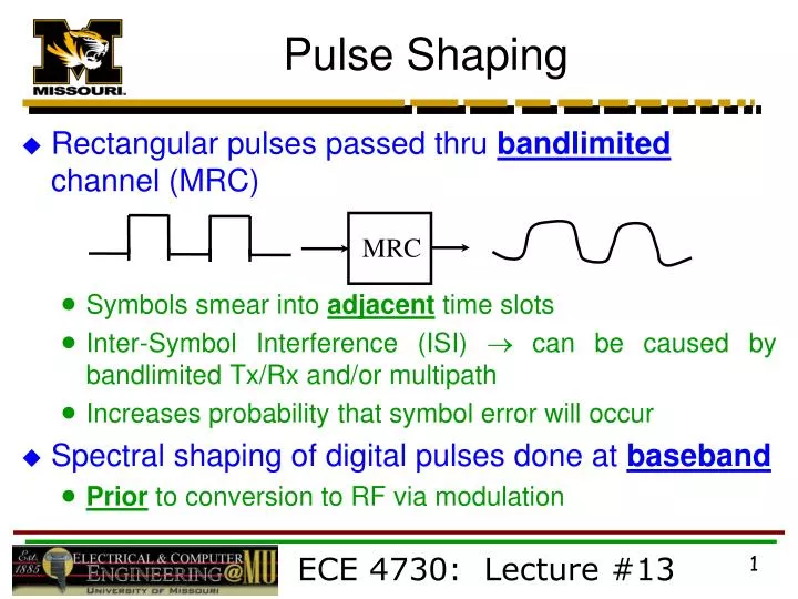
MRC. Pulse Shaping. Rectangular pulses passed thru bandlimited channel (MRC) Symbols smear into adjacent time slots Inter-Symbol Interference (ISI) can be caused by bandlimited Tx/Rx and/or multipath Increases probability that symbol error will occur

E N D
MRC Pulse Shaping • Rectangular pulses passed thru bandlimited channel (MRC) • Symbols smear into adjacent time slots • Inter-Symbol Interference (ISI) can be caused by bandlimited Tx/Rx and/or multipath • Increases probability that symbol error will occur • Spectral shaping of digital pulses done at baseband • Prior to conversion to RF via modulation ECE 4730: Lecture #13
PSD Sidelobes Tb ... V 0 1 1 f 0 1 / Tb = FNBW Pulse Shaping • Two primary goals : • Reduce ISI due to pulse smearing • Improve Bit Error Rate (BER) key performance measure for all digital communication systems • Reduce spectral width of signal • Improve BW efficiency • Achieve better control of ACI! • Even if MRC was NOT bandlimited it is impossible to transmit perfect “rectangular” pulse • PSD of rectangular pulse has INIFINITE bandwidth ECE 4730: Lecture #13
Pulse Shaping • Nyquist Criterion • Design overall response of system (Tx + MRC + Rx) so at every sampling instant in Rx (0/1 decision point) the response of all other symbols is zero • Leads to ideal “brick wall” filter in frequency domain • Cannot be achieved in practice due to infinite time domain pulse response ECE 4730: Lecture #13
Pulse Shaping • Raised Cosine (RC) Filter • Note RC Resistor Capacitor !! • Widely used & satisfies Nyquist criterion • Fig. 6.17 & 6.18, pg. 288 • a : rolloff factor ; as a 0 the filter “brick wall” • As a spectral BW of signal • Reduces signal BW and ACI desirable • Also increases sensitivity to timing errors undesirable ECE 4730: Lecture #13
Raised Cosine Filter Spectral Response Function 0 filter “brick wall” ECE 4730: Lecture #13
Raised Cosine Filter Time Domain Response 0 TDR sin x / x Note : TDR is 0 for nT no ISI ECE 4730: Lecture #13
Raised Cosine Filter • Symbol rate passed thru RC filter • Spectral efficiency is difficult to preserve in non-linear RF amplifiers (e.g. Class C) • Non-linear amplifier distorts baseband shape and increases spectral BW • Spectral regeneration • Require linear amplifiers for RC pulse shaping • Poor DC/RF conversion efficiency • Primary disadvantage ECE 4730: Lecture #13
Pulse Shaping • Gaussian Filter • Non-Nyquist filter used for pulse shaping to reduce spectral BW • Can be used with DC-RF efficient non-linear amplifiers when digital frequency modulation is used ECE 4730: Lecture #13
Gaussian Filter Time & Frequency Domain BOTH Have Gaussian Shape ECE 4730: Lecture #13
Gaussian Filter • As a spectral BW of signal • Primary advantage • However as a BER due to ISI as BW • Primary disadvantage • Gaussian filter only useful for limiting signal BW and NOT for mitigating ISI • Use when DC-RF efficiency of amplifier is major concern mobile unit !! • Non-linear Class C amplifiers with 80-90% DC-RF efficiencies ECE 4730: Lecture #13
Constellation Diagrams • Graphical representation of complex (A & q) digital modulation types • Provide insight into modulation performance • Modulation set, S, with M possible signals • Binary modulation M = 2 each signal = 1 bit of information • M-ary modulation M > 2 each signal > 1 bit of information ECE 4730: Lecture #13
1 0 1 t Constellation Diagrams • Example: Binary Phase Shift Keying (BPSK) for 0 t Tb Phase change between bits = 180° ! ECE 4730: Lecture #13
Constellation Diagrams • BPSK Example (continued) • Let basis signal • Then • N: dimension of vector space = # of basis signals required to represent S (here N = 1) • Plot amplitude & phase of S in complex vector space • Constellation Diagram “1” “0” ECE 4730: Lecture #13
Imaginary (Quadrature) Real (In-Phase) “0” “1” BPSK Signal Constellation BPSK ECE 4730: Lecture #13
Constellation Diagrams • Important Properties 1) Distance between signals related to how unique or different modulation waveforms are • Large separation distance “sparse” easy to discriminate good BER @ low SNR ( Eb / No) !! \Power Efficient • Note: Density w.r.t. # states / N ECE 4730: Lecture #13
Constellation Diagrams • Important Properties 2) Occupied BW as # signal states • Small separation distance “dense” more signal states/symbol more information/Hz !! \Bandwidth Efficient • Higher data rate for given signal BW • Greater bps per unit Hz ECE 4730: Lecture #13