Atmospheric Correction

1. Atmospheric Correction Sherry Palacios, MeloëKacenelenbogen, & John Livingston HQ2-O Workshop September 3, 2014

2. Talking Points • Atmospheric Correction Description • Overview of Tafkaa – Theory and Equations • Inputs and Outputs of Tafkaa • Uncertainty with Tafkaa • AATS-14 Data Related to Atmospheric Correction • Model Study of Aerosols • Problems and Perspectives

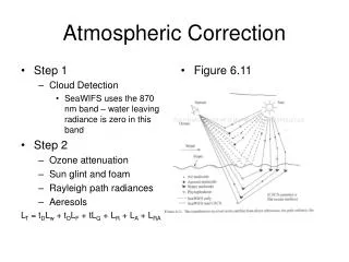
3. Atmospheric correction removes the contributions of surface glint and atmospheric scattering to obtain the water-leaving radiance from the measured total radiance sensor Atmospheric contribution is ~ 90 % of at-sensor radiance and varies due to aerosols, water vapor, ozone, gases, and other atmospheric constituents 80% of that atmospheric influence is due to aerosols (Meloë’s specialty) sky scattered scattering into IFOV scattered from sun to sensor sun glint sky glint reflected light scattered out of IFOV scattering out of IFOV Lw Total water-leaving radiance, Lr Radiance above the sea surface due to all surface reflection effects within the IFOV, Lp Atmospheric path radiance light path of water-leaving radiance water-leaving radiance outside IFOV, scattered toward sensor http://disc.sci.gsfc.nasa.gov/education-and-outreach/additional/science-focus/classic_scenes/11_classics_radiation.shtml

4. Atmospheric Correction Algorithms Used with Imaging Spectrometer (‘Hyperspectral’) Data for the Ocean • 6S (Second Simulation of the Satellite Signal in the Solar Spectrum) (Vermote et al. 1997) • ATREM (ATmosphericREMoval algorithm) (Gao et al. 1993 and Gao & Davis 1997) • Tafkaa(The Algorithm Formerly Known As ATREM) (Gao et al. 2000, Montes et al. 2001, and Montes et al. 2003)

5. Lt = total radiance or, “at-sensor radiance” L0 = L0 (l;q;f;q0;f0;ta;zsen;zsur) “atm. scattered radiance if radiance above sea surface is zero” Lsfc = Lsfc(l;q;f;q0;f0;W;ta;zsur) “direct & diffuse radiance reflected from surface” Lg = Lg(l;q;f;q0;f0;W;C;ta;zsur) “target radiance assuming Lambertian surface” t = t(l;q;ta;zsen;zsur) “transmission through atm. of Lsfc” t’ = t’(l;q;ta;zsen;zsur) “transmission through atm. of Lg” Lsa = L0 + Lsfc*t L’sa = Lsa * Tg Tg= transmission due to absorptive processes in gas Lw = water-leaving radiance nLw = normalized water-leaving radiance t0 = t0 (l;q0) single scattering diffuse transmittance fsol = earth-sun distance correction fob = out of band response correction fbrdf = Bi-directional reflectance distribution function correction m0 = cos(q0) “cosine of zenith sun angle” E0 = downward solar spectral irradiance at top of atm. td = downward transmittance through atm. to target Equations to Produce Geophysical Data Products Radiance (L) Lt = L0 + Lsfc*t + Lg*t’ Lt = Tg(L’sa+ Lg*t’) assume Lg = Lw nLw = Lw/( t0m0fsol)*fob* fbrdf Reflectance (r) rg≡ πLg / m0E0td Remote Sensing Reflectance (Rrs) Rrs = rg / π References on ‘Publications’ slide

6. The version of Tafkaa we use, uses pre-calculated look-up tables for various atmospheric scattering quantities; look-up tables include the specular effects of the air-water interface Atmospheric correction removes the contributions of surface glint and atmospheric scattering to obtain the water-leaving radiance from the measured total radiance variables acted on during atmospheric correction at-sensor radiance Lt = Tg(L’sa+ Lg* t’) water- leaving radiance

7. Inputs and Outputs of Tafkaa Inputs: housekeeping: image (Lt) & image header, image geometry, imager pointing, parameter set-up file atmospheric & surface parameters: gases (H2O, CO2, O3, N2O, CO, CH4, O2), column ozone, column water vapor, relative humidity, aerosol optical depth, aerosol model Outputs: atmospherically corrected image with units of either- reflectance, ρg remote sensing reflectance, Rrs or normalized water-leaving radiance, nLw Station 18 Station 17 October 28, 2011

8. Example Parameter File Aerosol model choice can strongly influence outcome (Standby for Meloë)

9. Raw Headwall Radiance Lt (100 * W m-2 nm-1 sr-1) A Comparison of Spectra: at-sensor, atmospherically corrected, and in-water at-sensor Lt nLw (W cm-2 nm-1 sr-1) TafkaanLw Station 17, Chl = 6.8 mg m-3 Station 18, Chl = 52.8 mg m-3 nLw (W cm-2 nm-1 sr-1) Tafkaa Parameters model tropospheric, tau550nm 0.11, ozone 0.269, column water vapor 1.25, relative humidity 80% in-water nLw

10. Tafkaa User Community • Users are typically from the hyperspectral, ocean color remote sensing community and include: • The HICO User’s Group (http://hico.coas.oregonstate.edu/publications/publications.shtml) • Naval Research Lab • Ocean color researchers using AVIRIS data (e.g. Bagheri 2011)

11. Uncertainty in the Data Products • Scant evidence in the literature of a robust sensitivity analysis of Tafkaa • Sensitivity analysis is part of this project and is currently being developed by Sherry, Meloë, John L., and Kirk • Evaluation of error propagation using Jacobian matrix approach being considered (e.g. Knobelspiesse et al. 2012). • Use of nLwvs. Rrs vs. Chlorophyll vs. Phytoplankton taxa as unit for sensitivity analysis. Topic is open to discussion with respect to best unit for estimating error propagation.

12. Some recent results from preliminary sensitivity analysis tau550 = 0.14, water vap= 1 cm, O3 = 0.269 atm*cm, wind speed = 2 m s-1 Station 17, Chl = 6.8 mg m-3 Urban Tropospheric RH RH HyperPro-groundtruth HyperPro-groundtruth HyperPro-groundtruth HyperPro-groundtruth Remote Sensing Reflectance (sr-1) Remote Sensing Reflectance (sr-1) Wavelength (nm) Wavelength (nm) Station 18, Chl = 52.8 mg m-3, “redtide” RH RH Urban Tropospheric Remote Sensing Reflectance (sr-1) Remote Sensing Reflectance (sr-1) Wavelength (nm) Wavelength (nm)

13. Publications Protocols: Bo-CaiGao, MJ Montes, Z Ahmad, CO Davis (2000) Atmospheric correction algorithm for hyperspectral remote sensing of ocean color from space. Appl. Optics 21(6):887 – 896 M. J. Montes, B.-C. Gao, and C. O. Davis (2001) A new algorithm for atmospheric correction of hyperspectral remote sensing data. Geo-Spatial Image and Data Exploitation II, Proceedings of the SPIE, 4383, 23-30 2001 April 16, SPIE'sAeroSense, Orlando, FL, USA M. Montes, B.-C. Gao, and C. O. Davis (2003) Tafkaa atmospheric correction of hyperspectral data. Imaging Spectrometry IX, Proceedings of the SPIE, 5159, 2003 August 6, SPIE's 48th Annual Meeting, San Diego, CA, USA The Manual: NRL Atmospheric Correction Algorithms for Oceans: Tafkaa User's Guide Marcos J. Montes, Bo-CaiGao, and Curtiss O. Davis 2004 NRL/MR/7230--04-8760 Background: Ahmad, Z, BA Franz, CR McClain, EJ Kwiatkowska, J Werdell, EP Shettle, & BN Holben (2010) New aerosol models for the retrieval of aerosol optical thickness and normalized water-leaving radiances from the SeaWiFS and MODIS sensors over coastal regions and open oceans. Appl. Optics 49(29): 5545 – 5560. Gao, B-C. KH Heidebrecht, & AFH Goetz (1993) Derivation of scaled surface reflectances from AVIRIS data. Remote Sens. Env. 44: 165 – 178. Gao, B-C & C Davis (1997) Development of a line-by-line based atmosphere removal algorithm for airborne and spaceborne imaging spectrometers. Imaging Spectrometry III, MR Descour & SS Shen eds. Proc. SPIE 3118: 132 – 141. Knobelspiesse, K, B Cairns, M Mishchenko, J Chowdhary, K Tsigaridis, B van Diedenhoven, W Martin, M Ottaviani, & M Alexandrov (2012) Analysis of fine-mode aerosol retrieval capabilities by different passive remote sensing instrument designs. Optics Express 20(19): 21457 – 21484 Vermote, EF, D Tanre, JL Deuze, M Herman, & JJ Morcrette (1997) Second simulation of the satellite signal in the solar spectrum, 6S: An overview. IEEE Transactions on Geoscience and Remote Sensing 35(3): 675 – 686. Topical: Patterson, KW & G Lamela (2011) Influence of aerosol estimation on coastal water products retrieved from HICO images. Ocean Sensing and Monitoring III. W Hou & R Arnone Eds. Proc. SPIE 8030:803005 1-9. Bagheri, S. (2011) Nearshore water quality estimation using atmospherically corrected AVIRIS data. Remote Sensing. 3:257 – 269.