Download
1 / 30
550 likes | 1.79k Views
Introduction to Laser Doppler Velocimetry. Ken Kiger Burgers Program For Fluid Dynamics Turbulence School College Park, Maryland, May 24-27. Laser Doppler Anemometry (LDA). Single-point optical velocimetry method. 3-D LDA Measurements on a 1:5 Mercedes-Benz

E N D
Introduction to Laser Doppler Velocimetry Ken Kiger Burgers Program For Fluid Dynamics Turbulence School College Park, Maryland, May 24-27
Laser Doppler Anemometry (LDA) • Single-point optical velocimetry method 3-D LDA Measurements on a 1:5 Mercedes-Benz E-class model car in wind tunnel Study of the flow between rotating impeller blades of a pump
Phase Doppler Anemometry (PDA) • Single point particle sizing/velocimetry method Droplet Size Distributions Measured in a Kerosene Spray Produced by a Fuel Injector Drop Size and Velocity measurements in an atomized Stream of Moleten Metal
Laser Doppler Anemometry • LDA • A high resolution - single point technique for velocity measurements in turbulent flows • Basics • Seed flow with small tracer particles • Illuminate flow with one or more coherent, polarized laser beams to form a MV • Receive scattered light from particles passing through MV and interfere with additional light sources • Measurement of the resultant light intensity frequency is related to particle velocity A Back Scatter LDA System for One Velocity Component Measurement (Dantec Dynamics)
LDA in a nutshell • Benefits • Essentially non-intrusive • Hostile environments • Very accurate • No calibration • High data rates • Good spatial & temporal resolution • Limitations • Expensive equipment • Flow must be seeded with particles if none naturally exist • Single point measurement technique • Can be difficult to collect data very near walls
Review of Wave Characteristics • General wave propagation • A = Amplitude • k = wavenumber • x = spatial coordinate • t = time • = angular frequency e = phase
Electromagnetic waves: coherence • Light is emitted in “wavetrains” • Short duration, Dt • Corresponding phase shift, e(t); where e may vary on scale t>Dt • Light is coherent when the phase remains constant for a sufficiently long time • Typical duration (Dtc) and equivalent propagation length (Dlc) over which some sources remain coherent are: • Interferometry is only practical with coherent light sources Sourcelnom (nm)Dlc White light 550 8 mm Mercury Arc 546 0.3 mm Kr86 discharge lamp 606 0.3 m Stabilized He-Ne laser 633 ≤ 400 m
Electromagnetic waves: irradiance • Instantaneous power density given by Poynting vector • Units of Energy/(Area-Time) • More useful: average over times longer than light freq. Frequency Range 6.10 x 10¹⁴ 5.20 x 10¹⁴ 3.80 x 10¹⁴
LDA: Doppler effect frequency shift • Overall Doppler shift due two separate changes • The particle ‘sees’ a shift in incident light frequency due to particle motion • Scattered light from particle to stationary detector is shifted due to particle motion
LDA: Doppler shift, effect I • Frequency Observed by Particle • The first shift can itself be split into two effects • (a) the number of wavefronts the particle passes in a time Dt, as though the waves were stationary… Number of wavefronts particle passes during Dt due to particle velocity:
LDA: Doppler shift, effect I • Frequency Observed by Particle • The first shift can itself be split into two effects • (b) the number of wavefronts passing a stationary particle position over the same duration, Dt… Number of wavefronts that pass a stationary particle during Dt due to the wavefront velocity:
LDA: Doppler shift, effect I • The net effect due to a moving observer w/ a stationary source is then the difference: Number of wavefronts that pass a moving particle during Dt due to combined velocity (same as using relative velocity in particle frame): Net frequency observed by moving particle
LDA: Doppler shift, effect II • An additional shift happens when the light gets scattered by the particle and is observed by the detector • This is the case of a moving source and stationary detector (classic train whistle problem) receiver lens Distance a scattered wave front would travel during Dt in the direction of detector, if u were 0: Due to source motion, the distance is changed by an amount: Therefore, the effective scattered wavelength is:
LDA: Doppler shift, I & II combined • Combining the two effects gives: • For u << c, we can approximate
LDA: problem with single source/detector • Single beam frequency shift depends on: • velocity magnitude • Velocity direction • observation angle • Additionally, base frequency is quite high… • O[1014] Hz, making direct detection quite difficult • Solution? • Optical heterodyne • Use interference of two beams or two detectors to create a “beating” effect, like two slightly out of tune guitar strings, e.g. • Need to repeat for optical waves P
Optical Heterodyne • Repeat, but allow for different frequencies…
How do you get different scatter frequencies? • For a single beam • Frequency depends on directions of es and eb • Three common methods have been used • Reference beam mode (single scatter and single beam) • Single-beam, dual scatter (two observation angles) • Dual beam (two incident beams, single observation location)
Dual beam method Real MV formed by two beams Beam crossing angle g Scattering angle q ‘Forward’ Scatter Configuration
Dual beam method (cont) Note that so:
Fringe Interference description • Interference “fringes” seen as standing waves • Particles passing through fringes scatter light in regions of constructive interference • Adequate explanation for particles smaller than individual fringes L
Gaussian beam effects A single laser beam profile • Power distribution in MV will be Gaussian shaped • In the MV, true plane waves occur only at the focal point • Even for a perfect particle trajectory the strength of the • Doppler ‘burst’ will vary with position Figures from Albrecht et. al., 2003
Non-uniform beam effects Particle Trajectory Centered Off Center DC AC DC+AC • Off-center trajectory results in weakened signal visibility • Pedestal (DC part of signal) is removed by a high pass filter after • photomultiplier Figures from Albrecht et. al., 2003
Multi-component dual beam ^ xg ^ xb Three independent directions Two – Component Probe Looking Toward the Transmitter
Sign ambiguity… • Change in sign of velocity has no effect on frequency Xg uxg> 0 beam 2 beam 1 uxg< 0
Velocity Ambiguity • Equal frequency beams • No difference with velocity direction… cannot detect reversed flow • Solution: Introduce a frequency shift into 1 of the two beams Xg Bragg Cell fb2 = fbragg+ fb beam 1 fb = 5.8 e14 beam 2 fb1 = fb New Signal If DfD < fbragg then u < 0 Hypothetical shift Without Bragg Cell
Frequency shift: Fringe description • Different frequency causes an apparent velocity in fringes • Effect result of interference of two traveling waves as slightly different frequency
Directional ambiguity (cont) DfD s-1 fbragg uxg (m/s) l = 514 nm, fbragg = 40 MHz and g = 20° Upper limit on positive velocity limited only by time response of detector
Velocity bias sampling effects • LDA samples the flow based on • Rate at which particles pass through the detection volume • Inherently a flux-weighted measurement • Simple number weighted means are biased for unsteady flows and need to be corrected • Consider: • Uniform seeding density (# particles/volume) • Flow moves at steady speed of 5 units/sec for 4 seconds (giving 20 samples) would measure: • Flow that moves at 8 units/sec for 2 sec (giving 16 samples), then 2 units/sec for 2 second (giving 4 samples) would give
Laser Doppler Anemometry Velocity Measurement Bias nth moment Mean Velocity Bias Compensation Formulas - The sampling rate of a volume of fluid containing particles increases with the velocity of that volume - Introduces a bias towards sampling higher velocity particles
Phase Doppler Anemometry The overall phase difference is proportional to particle diameter Multiple Detector Implementation The geometric factor, b - Has closed form solution for p = 0 and 1 only - Absolute value increases with y (elevation angle relative to 0°) - Is independent of np for reflection Figures from Dantec