Download
1 / 13
130 likes | 384 Views
CWB WRF/DART Ensemble Filter Assimilation System Process. Yun-Tien, Lin Hui Liu Ying-Hwa, Kuo. Introduction. WRF/DART is an ensemble filter data assimilation system including the Ensemble Adjustment Filter and other filters

E N D
CWB WRF/DART Ensemble Filter Assimilation System Process Yun-Tien, Lin Hui Liu Ying-Hwa, Kuo
Introduction • WRF/DART is an ensemble filter data assimilation system including the Ensemble Adjustment Filter and other filters • Many observation types can be assimilated: Conventional observations (radiosonde, aircrafts, satellite wind, etc.);Radar and GPS observations. • New model physics and observation types can be added easily without need of tangent and adjoint models.
Ensemble Adjustment Filter(Anderson, 2003) Assumption: Each observation can be handled sequentially. 1st step: Update forecast ensemble estimates of the observation * * * * * * * * * * º * * * * * * * * * * N (refractivity) N1 N10 • We can shift the ensemble mean closer to the observation’s value and reduce uncertainty of the ensemble. • Get ensemble analysis increments by differencing the forecast and updated ensemble members.
Ensemble Adjustment Filter(cont.) 2nd step: Update ensemble members of each model variable at each of the nearby model grid point sequentially. Lat qj • • • • • • o • • • • • • • • Lon Key: Regress the analysis increments of the observation at the observation location to nearby model variablesusing a joint ensemble statistics of qj with N ( T,q,Ps )
Ensemble Adjustment Filter(cont.) 2nd step: Linear regression of the observation increments to nearby model variables. For example: qj * * qj,10 * * * * * * * * * * * * * * * * * * * qj,1 * * * * * * * * * * o N (refractivity) N1 N10
Procedure : 1. wrfbdy_d01_mean_148178_21600 wrfinput_d01_mean_148178_21600 2. wrfbdy_148178_21600_1 wrfinput_d01_148178_21600_1 Prepare EnKF IC & BC ( prepare_ICBC.csh & 3dvar_ICBC.csh ) Transfer Observation Data ( gts.csh ) 1. obs_seq20060913 EnKF analysis ( cwbctl${day}.csh ) 1. Posterior_Diag.nc 2. Prior_Diag.nc Update New WRF IC & BC Data ( nodatafcst.csh & update_ICBC.csh ) 1. wrfbdy_d01 2. wrfinput_d01_enkf
WRF/DART script shell 1. Prepare ensemble initial and boundary condition run.csh ( / DATA / WPS ) prepare_ICBC.csh ( / DATA / IC_CWB ) 3dvar_ICBC.csh ( / DATA / IC_CWB ) 2. Transform CWB_gts observations to DART format files gts.csh ( / DART / model / wrf / work ) 3. Run DART_WRF and produce ensemble analyses cwbctl${day}.csh ( / DATA / work ) 4. Produce WRF IC & BC data from the mean/member of ensemble analyses nodatafcst.csh & update_ICBC.csh ( / DATA / UPDATE_ICBC )
Prepare ensemble initial and boundary condition • run.csh : to produce met_em data from WPS ex : met_em.d01.2006-09-13_00:00:00.nc 1. cp /DATA/WPS/namelist.wps to WPS directory 2. check the initial data and namelsit.wps • prepare_ICBC.csh : prepare mean WRF boundary and input data ex : wrfbdy_d01_mean_148178_21600 wrfinput_d01_mean_148178_21600 • 3dvar_ICBC.csh : produce ensemble WRF boundary and input data using wrf3dvar (temporarily, using global WRF later) ex : wrfbdy_148178_21600_1 ~ wrfbdy_148178_21600_32 wrfinput_d01_148178_0_1 ~ wrfinput_d01_148178_0_32 P.S. Currently, the single thread version of wrfvar.exe is used (update wrfvar2.1_2.1)
Transform CWB gts observations to WRF/DART • gts.csh : to transfer CWB gts data to DART data format ex : obs_seq20060913 • 1. prepare CWB gts data ( ex : obs_gts.3dvar_d01_2006091300, hourly) 2. transform CWB gts data to DART gts data ( ./gts_tf_dart ) ( ex : obs_seq06091300.gts, hourly ) 3. merge ( ./merge_obs_seq ) the CWB gts data files to one daily DART gts data (optional) ( ex : obs_seq20060913 )
Run DART_WRF and produce ensemble analysis • cwb.csh : to produce a sequential time dependency c shells for running multi-days assimilation ex : cwbctl13.csh or cwbctl14.csh for day 13 and 14. 1. prepare the namelist.input.cwb for WRF and input.nml.template.cwbctl for WRF/DART 2. check the ensemble boundary and input condition data directory 3. check the advance_model.csh file • Cwbctl13.csh : run DART to get the ensemble analysis for day 13 • ex : Posterior_Diag.nc and Prior_Diag.nc ensemble analysis; obs_seq.final final obs_seq data at observations’ locations 1. Posterior_Diag.nc : ensemble analysis data 2. Prior_Diag.nc : ensemble first guess data P.S. the single thread version of wrf.exe is used at the moment. (A new script is being developed to run WRF model in MPI mode together with DART to speed up WRF model integration)
input.nml.template.cwbctl • &filter_nml • async = 2, • adv_ens_command = "./advance_model.csh", • ens_size = 32, ensemble members • start_from_restart = .true., • output_restart = .true., • obs_sequence_in_name = "obs_seq.out", • obs_sequence_out_name = "obs_seq.final", • restart_in_file_name = "filter_ics", • restart_out_file_name = "filter_restart", • init_time_days = 148178, initial day from year 1600 • init_time_seconds = 0, initial second of the initial day • first_obs_days = 148177, start day • first_obs_seconds = 84601, start second (1/2 hour before analysis time, for 1-hour assimilation window only) • last_obs_days = 148178, end day • last_obs_seconds = 43200, end second (1/2 hour after analysis time)
Produce WRF IC & BC data from ensemble analyses for WRF forecast • nodatafcst_CWB.csh : to produce no-data forecast ex : wrfbdy_d01 and wrfinput_d01 1. prepare the initial data and link the WPS and WRF directory 2. check the namelist.wps and namelist.input file • update_ICBC.csh : extract model variables from the analysis and generate new wrfbdy and wrfinput data ex : wrfbdy_d01 and wrfinput_d01_enkf_$time 1. wrfbdy_d01 : the updated wrf boundary data 2. wrfinput_d01_enkf : the updated wrf initail data
WRF/DART CPU Time and Disk Space for a test case(CWB 45km grid, 1-hour cycling) Run IC_CWB directory: prepare_ICBC.csh : 3 minutes 1 cpu 3dvar_ICBC.csh : 1 hour, 8 node / total 8 cpus directory space : 15,967,344 Kbyte temperate dir disk space : 12,707,872 Kbyte • Run UPDATE_ICBC directory : nodatafocst.csh and update_ICBC.csh : 2 minutes 1 cpu directory space : 807,104 Kbyte Run work directory : cwbctl13.csh : 5 hours and 40 minutes 4 node / total 64 cpus directory space : 11,856,880 Kbyte Ensemble analysis directory space : 10,760,464 Kbyte Run real case forecast directory : enkf_wrf.cmd : 12 minutes 4 node / total 64 cpus • Total run WRF/DART time : 7 hours • Total run WRF/DART disk space : 55,000,000 Kbyte ( 55 GB ) (with MPI run of WRF model, the time can be reduced to 1-2 hours)