Download
1 / 64
640 likes | 783 Views
Issues on Spurious Behaviors. Universidad Complutense de Madrid March 18, 2014. Christos Agiakloglou University of Piraeus. Three topics on spurious behaviors. Spurious Correlations for stationary AR(1) processes with Apostolos Tsimbanos

E N D
Issues on Spurious Behaviors Universidad Complutense de Madrid March 18, 2014 Christos Agiakloglou University of Piraeus
Three topics on spurious behaviors • Spurious Correlations for stationary AR(1) processes with Apostolos Tsimbanos • The Balance between Size and Power with Charalambos Agiropoulos • Spurious Regressions for non-linear or time varying coefficient processes with Anil Bera
Spurious Behavior • Granger and Newbold (1974) set the cat among the pigeons with their simulations results showing that when two independent drift-free random walks are used in a simple linear regression, one ends up with significant t-statistic 76% of the time. • This phenomenon was introduced by Yule (1926) as a spurious correlation. • Agiakloglou and Tsimpanos (2012) examined the spurious correlation phenomenon for stationary processes and they found no evidence of spurious behavior using the true variance of the sample correlation coefficient of the two independent AR(1) processes. • However, it was left to Phillips (1986) to mathematically prove the Granger-Newbold simulation results, showing that the usual t-statistic does not have a limiting distribution. • Entorf (1997) consider random walk with drifts. • Granger, Hyung and Jeon (2001) found spurious results even for stationary independent AR(1) processes.
The story continues • Marmol (1995) who generalized the work of Phillips (1986) for high-order integrated processes, showed also that the Durbin Watson statistic will converge in probability to zero and therefore low values of this statistic are expected to appear in the presence of spurious regressions, a finding that was also indicated by Granger and Newbold (1974). • Agiakloglou (2009) showed that evidence of serially correlated errors will also appear in the case of two independent stationary AR(1) processes, not only in first moments but also in second defined by an ARCH(1) error structure. • Recall, that the presence of serially correlated errors in the context of spurious regression had also been investigated by Newbold and Davies (1978) for variables that were generated for non-stationary moving average processes. • Tsay (1999) also examined spurious regression for I(1) processes with infinite variance errors.
Two Examples • Harvey ( 1980) “Econometrics – Alchemy or science?” studied the relationship between rainfall and inflation rate in U.K.. • Ferson, Sarkissian and Simin (2003) “Spurious regression in financial Economics” found that many predictive stock return regressions in the literature, based on individual predicting variables, may be spurious.
Spurious Correlations for Stationary AR(1) ProcessesAn alternative approach for testing for linear association for two independent stationary AR(1) processes Story Number One
Spurious Correlations vs. Spurious Regressions • Two similar if not identical terms referring to the same phenomenon of obtaining false evidence about the existence of a linear relationship between two variables. • In the case of spurious correlations the analyst has no indication about the existence of such behavior, unless he or she has some a priori information about the relationship between these two variables, such that a high absolute value of the sample correlation coefficient will be considered very suspicious. • In the case of spurious regressions the analyst will have an indication such as low value of the Durbin-Watson as Granger and Newbold (1974) have pointed out, see also Marmol (1995) and Agiakloglou (2009). • More difficult to detect spurious correlations.
Testing for Linear Association • The test of zero correlation in population is based on the following hypotheses: H0: ρ = 0 against H1: ρ≠ 0 and it is implemented by the usual t statistic, i.e., where r is the sample correlation coefficient and T is the sample size. • The t statistic follows a t distribution with (T - 2) degrees of freedom and the null hypothesis will be accepted if its absolute value is less than the critical value.
Frequency Distribution of r • Yule (1926) studied the properties of the sample correlation coefficient of two random variables and noticed that the major factor which determines this spurious behavior is the shape of the frequency distribution of the correlation coefficient of the two series. • More precisely, if the distribution has a U shape it is certain that spurious correlations will arise. • Banerjee, A., Dolado, J., Galbraith, J. W. and Hendry, D. F. (1993) using Monte Carlo analysis, examined the frequency distribution of the correlation coefficient for various orders of integrated independent time series verifying Yule’s (1926) initial results. • They concluded:
I) Frequency Distribution of r • A) if the two series are stationary white noise processes, the frequency distribution of the correlation coefficient will be symmetric around zero and it will look like normal distribution. Frequency distribution for the correlation coefficient between two independent white noise processes (T=100& 10,000 replications)
II) Frequency Distribution of r • B) if the two processes are non-stationary I(1) processes, the frequency distribution of the correlation coefficient will be semi-ellipse. Frequency distribution for the correlation coefficient between two independent I(1) processes (T=100 & 10,000 replications)
III) Frequency Distribution of r • C) If the two processes are non-stationary I(2) processes, the frequency distribution has a U shape with values of -1 and +1 to be more likely to occur. Frequency distribution for the correlation coefficient between two independent I(2) processes (T=100 & 10,000 replications)
Frequency Distribution of t • Consider: • a) two independent white noise processes, • b) two independent I(1) random walk processes, i.e., Yt = Yt-1 + ut, • c) two independent non-stationary I(2) processes, i.e., Yt = 2Yt-1 – Yt-2 + ut, for sample size of 100 observations using 10,000 replications. • Besides the percentage of rejections of the null hypothesis, the value of the standard deviation of the t statistic strongly deviates from one for the two non-stationary cases as appose to the white noise case which remains unchanged with value of one, regardless of the sample size. • Note the scale of the graphical presentation is not the same.
Simulation results for spurious correlations for white noise and non-stationary I(1) & I(2) processes based on 10,000 replications
I) Frequency Distribution of t Frequency distribution for the t statistic between two independent white noise processes (T=100 & 10,000 replications)
II) Frequency Distribution of t Frequency distribution for the t statistic between two independent I(1) processes (T=100 & 10,000 replications)
III) Frequency Distribution of t Frequency distribution for the t statistic between two independent I(2) processes (T=100 & 10,000 replications)
Spurious correlations for AR(1) • Consider two independent AR(1) processes Xt and Yt generated from the following DGP: and • where the errors εxt and εyt are each white noise N(0, 1) processes independent of each other and the autoregressive parameters are allowed to take values of 0.0, 0.2, 0.5, 0.8 and 0.9. • Note that if φx = φy = 1, both processes are non-stationary random walk processes without drift, whereas if φx = φy = 0, both processes are white noise processes.
Simulation Results • Unlike the two non-stationary cases, previously discussed and especially the I(1) case, the percentage of rejections of the null hypothesis of zero correlation remains unchanged regardless of the sample size. • It is only affected by the magnitude of the autoregressive parameters. • We get more spurious results as the value of the autoregressive parameter increases. • For example, for φx = φy = 0.5, the null hypothesis is rejected approximately 13%, for the 5% nominal level, whereas for φx = φy = 0.9, this number becomes approximately 52%.
Percentage of rejections of the null hypothesis of zero correlation at the 5% nominal level (|t| > 1.96) for two independent stationary AR(1) processes based on 10,000 replications
I) Further Simulation Results • Frequency distribution for the correlation coefficient • Clearly, if the decision, as to whether or not spurious behavior exists, was based on the shape of the frequency distribution of the correlation coefficient, the analyst will have no indication in this case. • The frequency distribution for the correlation coefficient of two independent stationary AR(1) processes is symmetric around mean zero and it looks very similar to the white noise case previously presented.
Frequency Distribution of r Frequency distribution for the correlation coefficient between two independent AR(1)processes for φχ = φy= 0.5 (T=100 & 10,000 replications)
Frequency Distribution of r Frequency distribution for the correlation coefficient between two independent AR(1) processes for φχ = φy= 0.9 (T=100 & 10,000 replications)
II) Further Simulation Results • Frequency distribution for the t statistic • As in the case of non-stationary processes, the problem of spurious correlations appears because the value of the standard deviation of the t statistic for testing the null hypothesis of zero correlation is not one for all values of the autoregressive parameters. • Thus, although the frequency distribution for the t statistic is symmetric around mean zero, it becomes flatter than the standard normal distribution as the value of the autoregressive parameters increases. • The standard deviation of the t statistic is affected only by the values of the autoregressive parameters and not by the sample size.
Standard deviation of the t statistic for testing the null hypothesis of zero correlation for two independent stationary AR(1) processes based on 10,000 replications
Frequency Distribution of t Frequency distribution for the t statistic between two independent AR(1)processes for φχ = φy = 0.5 (T=100 & 10,000 replications)
Frequency Distribution of t Frequency distribution for the t statistic between two independent AR(1) processes for φχ = φy = 0.9 (T=100 & 10,000 replications)
Variance of r of two independent AR(1) processes • For two independent stationary AR(1) processes Xt and Yt generated by equations (2) and (3) with autocorrelation coefficients ρx and ρy respectively we have: and since we have which approximately is equal to:
Variance of r of two independent AR(1) processes • Hence, the variance of the sample correlation coefficient between the two independent stationary AR(1) series is approximately defined as: or equivalently as: • since ρx= φx and ρy= φy for AR(1) processes. • For more evidence about the proof of this variance see Bartlett (1935). • McGregor (1962) also verifies the existence of this variance by determining the approximate null distribution of the sample correlation coefficient of two stationary Markov chain processes using the steepest descents method proposed by Daniels (1954 and 1956).
Variance of r of two independent AR(1) processes • The degree of accuracy of this variance depends on three things: • a) on the sign of the autoregressive parameters • b) on the absolute magnitude of the two autoregressive coefficients and • c) on the sample size • One should expect less accuracy: • a) if φx and φy are both positive (or negative) • b) if their absolute magnitude is close to one and • c) if their sample size is small. • Therefore, it is interesting to investigate the accuracy of this variance in the context of spurious correlations for all positive values of the autoregressive parameters and for various sample sizes.
Simulation Results using the Var(r) of two independent AR(1) processes • Series of two independent AR(1) processes Xt and Ytpreviously defined are generated for values of the autoregressive parameter of 0.0, 0.2, 0.5, 0.8 and 0.9 and for sample sizes of 100, 500 and 1,000 observations. • Based on the sample correlation coefficient of these two series, the test for zero correlation is conducted by replacing the denominator of the usual t statistic by the square root of the variance previously defined. • The simulation results support no evidence of spurious correlations. • Empirical levels are close to nominal levels for moderate and large sample sizes.
Percentage of rejections of the null hypothesis of zero correlation at the 5% nominal level (|t| > 1.96) for two independent stationary AR(1) processes using the approximate variance of their sample correlation coefficient based on 10,000 replications
Further Simulation Results using the Var(r) of two indep. AR(1) processes • Frequency distribution for the corrected t statistic • The frequency distribution of the corrected t statistic for testing the null hypothesis of zero correlation using the variance of two independent AR(1) processes is very close to the standard normal distribution since the standard deviation of the t statistic is one for almost all cases.
Standard deviation of the t statistic for testing the null hypothesis of zero correlation for two independent stationary AR(1) processes using the approximate variance of their sample correlation coefficient based on 10,000 replications
Concluding Remarks • Using the approximate variance of the sample correlation coefficient of two independent stationary AR(1) processes, this study shows that the spurious behavior can be eliminated for large and moderate sample sizes, even for large values of the autoregressive parameter.
The Balance between Size and Power in testing for linear association for two stationary AR(1) processes Story Number Two
Sample Correlation Coefficient • Fisher(1915)has revealed some of the properties of the sample correlation coefficient, r, indicating that it is a biased estimator of the population correlation coefficient, ρ, for normal populations, proving also that Ε[r] = ρ – ρ(1 – ρ2)/2Ν. • See also Kenny and Keeping (1951) and Sawkins (1944). • Clearly, the bias is not a large number, taking into account that the correlation coefficient takes values from -1 to 1. • However, if one is concerned with the accuracy of the t – test for testing the null hypothesis of zero correlation, especially when the absolute value of the sample correlation coefficient is small, this bias may affect the variance and, therefore, the test.
The test Statistics Consider and using the following three t statistics:
Simulation Process • Consider two independent AR(1) stationary processes generated by the following DGP: and • where the errors and are white noise N(0,1) processes, independent of each other and the autoregressive parameters are allowed to take values of 0.0, 0.2, 0.5, 0.8 and 0.9. • Sample sizes of 50, 100, 500 and 1000 observations.
Percentage of rejections of the null hypothesis of zero correlation at the 5% nominal level (|t| > 1.96) for two independent stationary AR(1) processes based on 10,000 replications
Comments • Using the empirical values of the autoregressive parameters we are getting better size for large values of the autoregressive parameter. • This is probably due to the fact that the estimates were not so close to the true large values of the autoregressive parameters for small and moderate sample sizes. • For example, for 0.9 and for T = 100, the mean values of the estimates were 0.8622 and 0.8614.
Mean values of the estimates of the autoregressive parameters of the AR(1) processes based on 10,000 replications
Power of the test • Consider two linearly dependent AR(1) processes Xtand Ytfor t = 1, 2, …, T, such that: • where is their correlation coefficient. • Using matrix notation, we may write: • where the errors and are white noise N(0, 1) processes, but not independent of each other.
Simulation Process • Equivalently, using matrices the former equation can be expressed as a VAR(1) model: where and are vectors with being a matrix. • It can be showed that: • where and are the covariance matrices of and respectively defined as: and • where and are the variances of and , respectively, defined by an AR(1) process, or is their covariance and or is the covariance of the error terms with unit variances.
Simulation Process – Cont. I • Using vectorization, the above equation becomes as: • where stands for vectorisation, ⊗ is the Kronecker product and is the identity matrix. • It is easy to show that the equation can be written precisely as: • from which the desired correlation ρ, between the two series, is determined by the following equation:
Simulation Process – Cont. II • Hence, to generate two dependent AR(1) processes with desired correlation , we need to generate random errors and with unit variances and correlation given by:
Percentage of rejections of the null hypothesis of zero correlation at the 5% nominal level (|t| > 1.96) for two dependent stationary AR(1) processes based on 10,000 replications
Percentage of rejections of the null hypothesis of zero correlation at the 5% nominal level (|t| > 1.96) for two dependent stationary AR(1) processes based on 10,000 replications
Percentage of rejections of the null hypothesis of zero correlation at the 5% nominal level (|t| > 1.96) for two dependent stationary AR(1) processes based on 10,000 replications
Comments • The test has low power for small and moderate sample sizes, especially for low values of the correlation coefficient, a result that has been also indicated by Zimmerman et. al. (2003) for normal populations. • However, as the sample size increases the power of the test also increases, regardless of the values of ρ and φ. • In general the classical t test has larger power than the other two tests. The difference is obvious for large values of the autoregressive parameter, low values of the correlation coefficient and small sample size. • For example, for T = 100, the null hypothesis is rejected 60.5% for ρ=0.2 and φ=0.9 using the classical t test, as opposed to 4.9% and 9.1% using the t'and the t'' statistic respectively. • For small values of the autoregressive parameters the power of the test is very similar for all three cases, regardless of the value of the correlation coefficient. • On the other hand, the test has larger power using the t'' rather than the t'statistic for all cases.