Download

1 / 19
200 likes | 350 Views
Continuous Distributions. ch3. A random variable X of the continuous type has a support or space S that is an interval(possibly unbounded) or a union of intervals, instead of a set of real numbers (discrete points).

E N D
A random variable X of the continuous type has a support or space S that is an interval(possibly unbounded) or a union of intervals, instead of a set of real numbers (discrete points). • The probability density function(p.d.f.) of X is an integrable function f(x) satisfying: • f(x)>0, x ∈S. • ∫Sf(x)dx= 1, • P(X∈A) = ∫Af(x)dx, where A ⊂S. • Ex.3.2-1: Assume X has the p.d.f. • P(X>20)=? • The distribution function of X is (cumulative distribution function) (c.d.f.) If the derivative F’(x) exists,
Zero Probability of Points • For the random variable of the continuous type, the probability of any point is zero. • Namely, P(X=b)=0. • Thus, P(a≤X≤b) = P(a<X<b) = P(a≤X<b) = P(a<X≤b) = F(b)-F(a). • For instance, • Let X be the times between calls to 911. 105 observations aremade to construct a relative frequent histogram h(x). • It is compared with the exponential model • in Ex3.2-1. 30 17 65 8 38 35 4 19 7 14 12 4 5 4 2 7 5 12 50 33 10 15 2 10 1 5 30 41 21 31 1 18 12 5 24 7 6 31 1 3 2 22 1 30 2 13 12 129 28 6 5063 5 17 11 23 2 46 90 13 21 55 43 5 19 47 24 4 6 27 4 6 37 16 41 68 9 5 28 42 3 42 8 52 2 11 41 4 35 21 3 17 10 16 1 68 105 45 23 5 10 12 17
(Dis)continuity, Differentiable, Integration • Ex3.2-4: Let Y be a continuous random variable with p.d.f. g(y)=2y, 0<y<1. • The distribution function of Y is • P(½≤Y≤¾)=G(¾)-G(½)=5/16. • P(¼≤Y<2)=G(2)-G(¼)=15/16. • Properties of a continuous random variable: • The area between the p.d.f. f(x) and x-axis must equal 1. • f(x) is possibly unbounded (say, >1). • f(x) can be discontinuous function (defined over a set of intervals), • However, its c.d.f. F(x) is always continuous since integration. • It is possible that F’(x) does not exist at x=x0.
Mean, Variance, Moment-generating Fn • Suppose X is a continuous random variable. • The expected value of X, the mean of X is • The variance of X is • The standard deviation of X is • The moment-generating function of X, if it exists, is • The rth moment E(Xr) exists and is finite ⇒E(Xr-1), …, E(X1) do. • The converse is not true. • E(etX) exists and is finite –h<t<h ⇒all the moments do. • The converse is not necessarily true. • Ex3.2-5: Random variable Y with p.d.f. g(y)=2y, 0<y<1. (Ex3.2-4)
Percentile (π) and Quartiles • Ex.3.2-6: X has p.d.f. f(x)=xe-x, 0≤x<∞. • The (100p)th percentiles a number πp s.t. the area under f(x) to the left of πp is p. • The 50thpercentileis called the median: m = π.5. • The 25th and 75thpercentiles are called the firstand thirdquartiles. • Namely, π.25= q1, π.75= q3, and m = π.5= q2 the second quartile. • Ex: X with p.d.f. f(x)=1-|x-1|, 0≤x<2. To find 32rd percentile π.32 is to solve F(π.32)=.32 ∵F(1)=.5>.32 To find 92rd percentile π.92 is to solve F(π.92)=.92
More Example • Ex3.2-8: X has the p.d.f. f(x)=e-x-1, -1<x<∞. • The median m = π.5 is
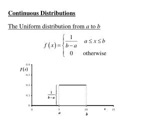
Uniform Distribution • Random variable X has a uniform distributionif its p.d.f. equals a constant on its support. • If the support is the interval [a, b], then p.d.f. ⇒ • This distribution, denoted as U(a, b), is also referred to as rectangular due to the shape of f(x). • The mean, variance, distribution function and moment-generating function are • Pseudo-random number generator: a program applies simple arithmetical operations on the seed (starting number) to deterministically generate a sequence of numbers, whose distribution follows U(0, 1). • Table IX on p.695 shows an example of these (random) numbers*104. • Ex.3.3-1: X has p.d.f. f(x)=1/100, 0<x<100, namely U(0,100). • The mean and variance are μ=(0+100)/2=50, σ2=10000/12. • The standard deviation is , 100 times of U(0,1).
Exponential Distribution • The waiting (inter-change) times W between successive changes whose number X in a given interval is a Poisson distributionis indeed an exponential distribution. • Such time is nonnegative ⇒the distribution function F(w)=0 for w<0. • For w ≥0, F(w) = P(W≤w) = 1 -P(W>w) = 1 -P(no changes in [0, w]) = 1 –e–λw, • For w>0, the p.d.f. f(w) = F’(w) = λe–λw⇒ • Suppose λ=7, the mean number of changes per minute; ⇒θ= 1/7, the mean waiting time for the first (next) change. • Ex3.3-2: X has an exponential distribution with a mean of θ=20.
Examples • Ex.3.3-3: Customers arrivals follow a Poisson process of 20 per hr. • What is the probability that the shopkeeper will have to wait more than 5 minutes for the arrival of the first (next) customer? • Let X be the waiting time in minutes until the next customer arrives. • Having awaited for 6 min., what is the probability that the shopkeeper will have to wait more than 3 min. additionally for the new arrival? • Memory-less, forgetfulness property! • Percentiles: • To exam how close an empirical collection of data is to the exponential distribution, the q-qplot (yr,πp) from the ordered statistics can be constructed, where p=r/(n+1), r=1,2,…,n. • If θis unknown, πp=-ln(1-p) can be used in the plot, instead. • As the curve ≈a straight line, it matches well. (Slope: an estimate of 1/θ)
Gamma Distribution F(w) • Generalizing the exponential distribution, the Gamma distribution considers the waiting time W until the αth change occurs, α≥1. • The distribution function F(w) of W is given by • Leibnitz's rule: • The Gamma function is defined by F’(w) generalized factorial
Fundamental Calculus • There are some formula from Calculus: • Generalized integration by parts (also ref. p.666): • Formula used in the Gamma distribution: • Pf: • Suppose • Then, a = m+1 : • By the induction hypothesis, the equation holds! α=1:
Chi-square Distribution • A Gamma distribution with θ=2, α=r/2, (r∈N) is a Chi-square distribution with r degrees of freedom, denoted as χ2(r). • The mean μ=r, and variance σ2=2r. • The mode, the point for the maximal p.d.f., is x=r-2 • Ex.3.4-3: X has a chi-square distribution with r=5. • Using Table IV on p.685 P(X>15.09)1-F(15.09)=1-0.99=0.01. P(1.145≦X≦12.83)=F(12.83)-F(1.145)=0.975-0.05=0.925. • Ex.3.4-4: X is χ2(7). Suppose there are two constants a & b s.t. P(a<X<b)=0.95. ⇒One of many possible is a=1.69 & b=16.01 • Percentiles: • The 100(1-α) percentile is • The 100αpercentile is f(x)
Distributions of Functions of Random Variable • From a known random variable X, we may consider another Y = u(X), a function of X, and want to know Y’s distribution function. • Distribution function technique: • We directly find G(y) = P(Y≤y) = P[u(X)≤y], and g(y)=G’(y). • E.g., finding the gamma distribution from the Poisson distribution. • Also, N(μ,σ2) ⇒N(0,1), and N(μ,σ2) ⇒χ2(1). • It requires the knowledge of the related probability models. • Change-of-variable technique: • Find the inverse function X=v(Y) from Y=u(X), and • Find the mapping: boundaries, one-to-one, two-to-one, etc. • It requires the knowledge of calculus and the like.
Distribution Function Technique G(w)= g(w)= • Ex: [Lognormal] X is N(μ,σ2). If W=eX, G(w)=?, g(w)=? • Ex3.5-2: Let w be the smallest angle between the y-axis and the spinner, and have a uniform distribution on (-π/2, π/2). y (0,1) w <=Cauchy p.d.f. g(x) x Both limits ⇒E(x) does not exist
Change-of of-variable Technique • Suppose X is a R.V. with p.d.f. f(x) with support c1< x < c2. • Y=u(X) ⇔the inverse X=v(Y) with support d1< y < d2. • Both u and v are conti. increasing functions, and d1=u(c1), d2=u(c2). • Suppose both u and v are conti. decreasing functions: • The mapping of c1< x < c2 would be d1> y > d2 • Generally, the support mapped from. G(y)= g(y)= Ex4.5-1 is an example. G(y)=…= g(y)=G’(y)
Conversions: Any ⇔ U(0,1) • Thm.3.5-2: X has F(x) that is strictly increasing on Sx={x: a<x<b}.Then R.V. Y, defined by Y=F(X), has a distribution U(0,1). • Pf: The distribution function of Y is • The requirement that F(x) is strictly increasing can be dropped. • It will take tedious derivations to exclude the set of intervals as f(x)=0. • The change-of-variable technique can be applied to the discrete type R.V. • Y=u(X), X=v(Y): there exists one-to-one mapping. • The p.m.f. of Y is g(y)=P(Y=y)=P[u(X)=y]=P[X=v(y)]=f[v(y)], y∈Sy. • There is no term “|v’(y)|”, since f(x) presents the probability.
Examples • Ex.3.5-6: X is a Poisson with λ=4. • If Y=X1/2, X=Y2, then • When the transformation Y=u(X) is not one-to-one, say V=Z2. • For instance, Z is N(0,1): -∞<z<∞, 0≤v<∞. [2-to-1 mapping] • Each interval (case) is individually considered. • Ex.3.5-7: X has p.d.f. f(x)=x2/3, -1<x<2. • If X=Y1/2, Y=X2, then 0≤y<4: • -1 < x1< 0 ⇔0 ≤y1< 1 • 0 ≤x2< 1 ⇔0 ≤y2< 1 • 1 ≤x3< 2 ⇔1 ≤y3< 4 G(v)= g(v)=
How to find E(X) & Var(X) now • Ex3.6-6: Find the mean and variance of X in previous example. • Ex3.6-7: Reinsurance companies may agree to cover the wind damages that ranges between $2 and $10 million. • X is the loss in million and has a distribution function: • If losses beyond $10 is set as $10, then • The cases (x>10) will all be attributed to x=10: P(X=10)=1/8. F(x)= μ=E(X) σ2=E(X2)-μ2