Download
1 / 71
810 likes | 1.45k Views
Continuous Distributions. The Uniform distribution from a to b. The Normal distribution (mean m , standard deviation s ). The Exponential distribution. Weibull distribution with parameters a and b . The Weibull density, f ( x ). ( a = 0.9, b = 2). ( a = 0.7, b = 2).

E N D
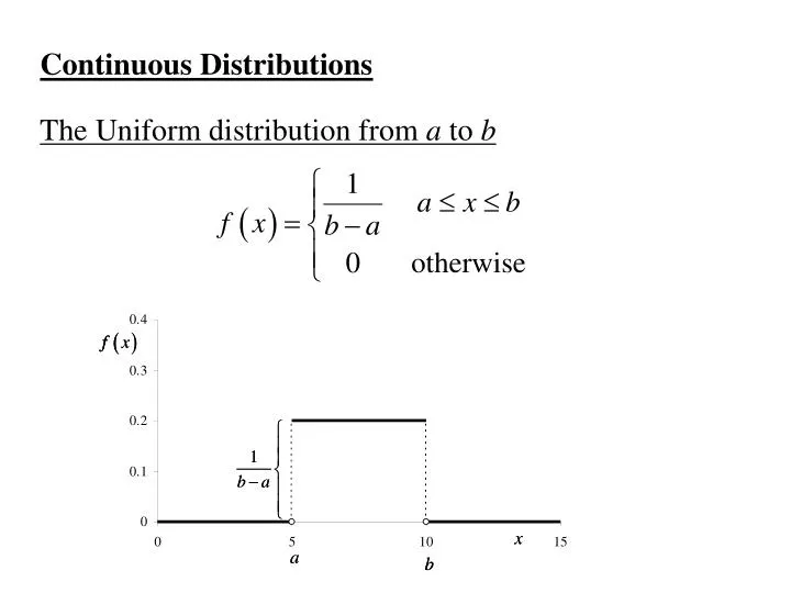
Continuous Distributions The Uniform distribution from a to b
The Weibull density, f(x) (a= 0.9, b= 2) (a= 0.7, b= 2) (a= 0.5, b= 2)
The Gamma distribution Let the continuous random variable X have density function: Then X is said to have a Gamma distribution with parameters aand l.
Let X denote a discrete random variable with probability function p(x) (probability density function f(x) if X is continuous) then the expected value of X, E(X) is defined to be: and if X is continuouswith probability density function f(x)
Interpretation of E(X) • The expected value of X, E(X), is the centre of gravity of the probability distribution of X. • The expected value of X, E(X), is the long-run average value of X. (shown later –Law of Large Numbers) E(X)
Example: The Uniform distribution Suppose X has a uniform distribution from a to b. Then: The expected value of X is:
Example: The Normal distribution Suppose X has a Normal distribution with parameters mand s. Then: The expected value of X is: Make the substitution:
Hence Now
Example: The Gamma distribution Suppose X has a Gamma distribution with parameters aand l. Then: Note: This is a very useful formula when working with the Gamma distribution.
The expected value of X is: This is now equal to 1.
Thus if X has a Gamma (a ,l) distribution then the expected value of X is: Special Cases: (a ,l) distribution then the expected value of X is: • Exponential (l) distribution:a = 1, l arbitrary • Chi-square (n) distribution:a = n/2, l = ½.
Definition Let X denote a discrete random variable with probability function p(x) (probability density function f(x) if X is continuous) then the expected value of g(X), E[g(X)] is defined to be: and if X is continuouswith probability density function f(x)
Example: The Uniform distribution Suppose X has a uniform distribution from 0to b. Then: Find the expected value of A = X2. If X is the length of a side of a square (chosen at random form 0 to b) then A is the area of the square = 1/3 the maximum area of the square
Example: The Geometric distribution Suppose X (discrete) has a geometric distribution with parameter p. Then: Find the expected value of XA and the expected value of X2.
Recall: The sum of a geometric Series Differentiating both sides with respect to r we get: Differentiating both sides with respect to r we get:
Thus This formula could also be developed by noting:
To compute the expected value of X2. we need to find a formula for Note Differentiating with respect to r we get
implies Thus
Definition Let X be a random variable (discrete or continuous), then the kthmoment of X is defined to be: The first moment of X , m = m1 = E(X) is the center of gravity of the distribution of X. The higher moments give different information regarding the distribution of X.
Definition Let X be a random variable (discrete or continuous), then the kthcentralmoment of X is defined to be: wherem = m1 = E(X) = the first moment of X .
The central moments describe how the probability distribution is distributed about the centre of gravity, m. = 2ndcentral moment. depends on the spread of the probability distribution of X about m. is called the variance of X. and is denoted by the symbolvar(X).
is called the standard deviation of X and is denoted by the symbols. The third central moment contains information about the skewness of a distribution.
The third central moment contains information about the skewness of a distribution. Measure of skewness
The fourth central moment Also contains information about the shape of a distribution. The property of shape that is measured by the fourth central moment is called kurtosis The measure ofkurtosis
Example: The uniform distribution from 0 to 1 Finding the moments
Thus The standard deviation The measure of skewness The measure of kurtosis
Rules: Proof The proof for discrete random variables is similar.
Proof The proof for discrete random variables is similar.
Proof The proof for discrete random variables is similar.