Download
1 / 34
340 likes | 508 Views
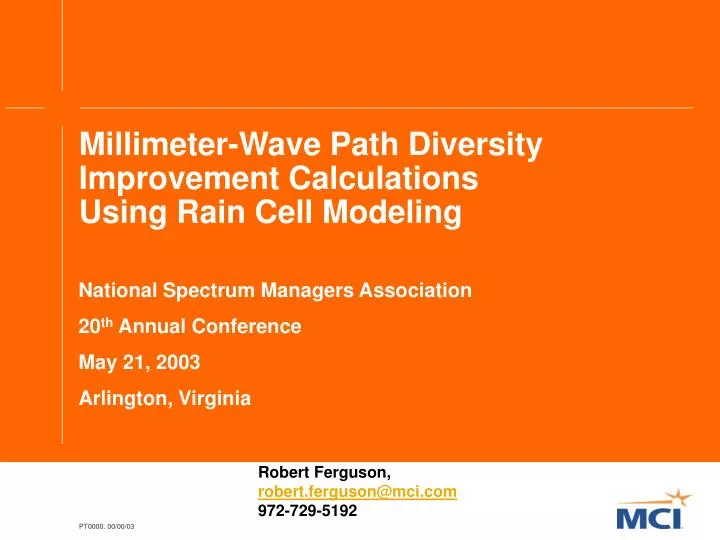
Millimeter-Wave Path Diversity Improvement Calculations Using Rain Cell Modeling. National Spectrum Managers Association 20 th Annual Conference May 21, 2003 Arlington, Virginia. Robert Ferguson, robert.ferguson@mci.com 972-729-5192. Outline. The Problem Overview Of The Rain Cell Model

E N D
Millimeter-Wave Path Diversity Improvement Calculations Using Rain Cell Modeling National Spectrum Managers Association 20th Annual Conference May 21, 2003 Arlington, Virginia Robert Ferguson,robert.ferguson@mci.com972-729-5192
Outline • The Problem • Overview Of The Rain Cell Model • Simulation Methodology And Assumptions • Path Diversity Improvement Factor (PDIF) • Definition • Interpretations • Simulation Results – Selected Examples • Final Comments
Problem:A Robust Millimeter-Wave System Extends A Fiber Network. Every Radio Node Has One Or More Backup Links, Improving Reliability During Rain Fade Events. How Effective Is This “Path Diversity”? There Will Be Some Correlation Of Rain Fading On Paths A & B – How Much ? Radio Link 99.995% 99.999% To Customer ? A C 0.005% > to 0.001% ? Fiber Network B 99.995% = Fiber or Radio Node
Fading Correlation: A Meteorology, Geometry, Radio ProblemThe Shape, Size, Orientation, And Variation In Rain Rate Intensity Of Rain Cell Distributions In A Region, In Relation To The Radio Path Distances, Angles And Operating Frequencies, Must Be Considered • If Critical Rain Cells Are Large Compared To Paths And Occur Frequently, Fading Will Be More Correlated (Cell 1) • The Angle Between Paths To A Node Is Important, With More Correlation On Smaller Angles (Cell 2 & Cell 3) 2 C A 3 B 1 To Estimate The Effectiveness Of Path Diversity, A Model Of Rain Cell Characteristics Is Needed
Rain Cell Modeling OverviewBased on Capsoni Model,Radio Science Volume 22, Number 3, Pages 387-404, May-June 1987 • A “Rain Cell” is defined as connected region where the rain intensity (mm/hr) exceeds a given threshold • Rain cells have intensity and spatial characteristics which have been statistically modeled based on experimental data collected using meteorological radar • In the Capsoni Model, an elliptical rain cell is specified by: • Peak rain rate (mm/hr) - Rm - at cell center • Characteristic radius at which intensity falls by “1/e” of Rm • Elliptical cell axial ratio = Minor Axis/Major Axis • Orientation of ellipse (“tilt”) w.r.t. coordinate system • The Capsoni Model specifies a cell “1/e radius” statistical distributionfor an assumed cell peak rain rate; on average, higher peak rate rain cells have smaller “1/e radii”
Rain Cell Modeling Overview - continuedBased on Capsoni Model,Radio Science Volume 22, Number 3, Pages 387-404, May-June 1987 • Intuitively, rain cell statistical characteristics are related to the point rain rate cumulative time distributions specified by the Crane and ITU rain zone classification systems • Capsoni, et al, describe a methodology to convert the point rainfall rate rate time distribution data to the statistical factors necessary to complete a rain cell model which can reproduce the assumed point rainfall rate statistics • This model can be used to evaluate the rain fade correlation effects on example desired/interfering path geometries, as well as the “path diversity” effects to be discussed
Elliptical Rain Cell Model Geometry Cell Defined by Rm (Peak Rain Rate mm/hr) and rho_x, rho_y Minor Axis (0.0, rho_y) (1/e * Rm) Rain Rate Isopleth (rho_x, 0.0) Major Axis R = Rm * exp (-sqrt( xf*xf + yf*yf)) where: xf = x/rho_x and yf = y/rho_y By definition, at (rho_x,0.0), R = 1/e * Rm at (0.0,rho_y), R = 1/e * Rm Intensity falls off to infinity Cell Axial Ratio = Minor Axis/Major Axis (on any rain rate isopleth) = rho_y/rho_x< 1.0 9
Rain Cell Ellipse Major Axis “Split Geometry” Illustration Proposed Modification To Model – To Account For Cell Asymmetry For Interference Analysis And Path Diversity ProblemsModel Ellipse Extends to Infinity on One Side of Major Axis y2 100 mm/hr Isopleth y1 x2 Major Axis x1 Assume only one portion of the split rain cell is “active” If rain at origin, also at x1 and y1 If NO rain at origin, rain at x2 and y2 Origin As drawn, Minor/Major Axis Ratio = ~ 0.5
Exponential Fall-Off Of Rain Rate From Cell Center (For Circular Rain Cell, rho(x,y) = Distance from Center) Area Of >50 mm/hr Cell PeakArea 50 mm/hr 0.0 km^2 100 1.0 150 2.0 200 2.8 250 3.4 300 3.8 350 4.1
Example Of A Rain Cell – Peak Rate Rm=200 mm/hr Typical (*) Size & Shape Cell Axial Ratio ~ 0.5 rho_x = 0.96 km rho_y = 0.48 km y 0 mm/hr at infinity 0.96 km Rm = 200 mm/hr 0.96 km x 1.92 km 27 mm/hr 45 mm/hr (*) In Capsoni Rain Cell Model, Size And Shape Are Varied Statistically About Average / Median Values Rm/e = 74 mm/hr 121 mm/hr
Comments On Simulation Results • All Examples Are Based On The “Test Rain Zone” Point Rainfall Statistics ApproximationTo ITU-R Zone N (Florida) – Highest Rates, Continental US (35 mm/hr @ 0.10%, 95 mm/hr @ 0.01%, 180 mm/hr @ 0.001%) • All Examples Assume H-Polarization • To Allow For Rain Cell Asymmetry, The Capsoni Model Has Been Modified By Adding “Cell Splitting” • Only Rain Cells With Peak Rain Rates (Rm) > 50 mm/hr And Elliptical Axial Ratio Less Than The Median (0.56) May Be Split; Randomly, One-Half Of These Cells Are Split Along The Major Axis. Each Half Of The Cell Is Used Separately • Results Will Change Somewhat With Differing “Split Criteria” • For Fades Occurrences Of Small Times (e.g. 0.001%), Reliance Of Any Model To Predict Improvement Factors Is Questionable - And Difficult To Validate By Measurement • The Simulation Evaluates A Single Rain Cell At A Time; The Model Is Likely More Valid For Shorter Paths That Would Be “Under The Influence” Of A Single Cell
Rain Rate Simulation - Random Factors Follow Model StatisticsFade Correlation Statistics Are Accumulated As Simulation Runs Generate random rain cells, following rain zone statistics, within Simulation Radius Simulation Radius Random Cells Factors: Peak Rain Rate - Rm Cell Radius - rho Location of Cell Center Axial Ratio Major Axis Tilt Angle Cell Split Criteria Path A Path B Virtual Rain Gauges Simulation should reproduce the point rain rate statistics assumed 11
Two-Path Fading Time MatrixDescribes Joint Fade Probability, Thus “Fade Correlation” Path A Fade Increments - In dB 0.0 1.0 2.0 3.0 4.0 5.0 6.0 7.0 8.0 9.0 10.0 11.0 12.0 13.0 … > 40.0 0.0 1.0 2.0 3.0 4.0 5.0 6.0 7.0 8.0 9.0 10.0 11.0 12.0 13.0 … >40.0 Note: The Sum of All Times In The Matrix Represents All Joint Fading Conditions Path B Fade Increments - In dB Note: One matrix would apply to two paths with specific geometry, frequency and rain zone statistics Entry Indicates Percentage of Time That: Path A Is In Fade Between 5.0 dB and 6.0 dB AND Path B Is In Fade Between 9.0 dB and 10.0 dB
Fading Correlation Using Two-Path Fading Time Matrix Path A Fade Increments – In dB F>35.0 dB 0 1 2 3 4 … 34 Sum Of TimesBeyond Line = 0.0033% 0 1 2 3 4 … 28 Path B Fade Increments – In dB Sum Of TimesBelow Line = 0.0354% In This Area, Sum Of Times = 0.0023% F>29.0 dB Fa > 35.0 & Fb > 29.0
Definition Of Path Diversity Improvement Factor – For This Presentation • Other “Improvement Factors”: Space Diversity, Polarization Diversity, Frequency Diversity, … • Path Diversity Improvement Factor - PDIF • Assume Path A Has A Critical Fade Depth Fa, Path B Has A Critical Fade Depth Fb • Based On Measured (Or Simulated) Fading Statistics • On Path A, (Fade > Fa) Occurs For Time = TA(F>Fa) • On Path B, (Fade > Fb) Occurs For Time = TB(F>Fb) • Jointly, Path A (Fade >Fa) And Path B (Fade >Fb) For Time = TAB(Fa,Fb) • Then, Assuming Either Path A Or Path B Can Provide “Service” If (Fade <= Critical), The Effectiveness Of Path Diversity Can Be Measured By Comparing Composite Performance To Either Path A or Path B Performance Alone: • PDIF(A/B) = TA(F>Fa)/ TAB(Fa,Fb) - “Path A Improved By Path B Diversity” • PDIF(B/A) = TB(F>Fb) / TAB(Fa,Fb) - “Path B Improved By Path A Diversity”
An Example Of Path Diversity Improvement • Two 28 GHz Paths Provide Redundant Traffic Paths To A Site; • Path A – 1.5 km, Critical Fade Margin Of 35.0 dB • 0.0033% = TA(F>35.0) – Time Of Predicted Rain Fade > 35.0 dB • Path B - 3.0 km, Critical Fade Margin Of 29.0 dB • 0.0354% = TB(F>29.0) – Time Of Predicted Rain Fade > 29.0 dB • Angle Between The Paths Is 135 Degrees • The Predicted Time When Both Paths Are Simultaneously Below Critical FM • 0.0023% = TAB(35.0,29.0) • Path Diversity Improvement Factors • 1.4= PDIF(A/B) = TA(F>35.0)/TAB(35.0,29.0)–Path A “Improved” By B Diversity • 15.3= PDIF(B/A) = TB(F>29.0)/TAB(35.0,29.0)–Path B “ By A Diversity B =3.0 km / 29 dB Customer A =1.5 km / 35 dB 135 Deg
Interpretation Of PDIF Using Two-Path Fading Time Matrix Path AFade Increments – In dB F>35.0 dB 0 1 2 3 4 … 34 Sum Of TimesBeyond Line = 0.0033% 0 1 2 3 4 … 28 Path B Fade Increments – In dB • PDIF(A/B) = 0.0033/0.0023 = 1.4 Sum Of TimesBelow Line = 0.0354% In This Area, Sum Of Times = 0.0023% F>29.0 dB • PDIF(B/A) = 0.0354/0.0023 = 15.3
Path Diversity Improvement – Decibel Interpretation • Path Diversity “Improves” The Reliability That Each Individual Path Can Provide, As Expressed By The PDIF • The Diversity Improvement Can Also Be Expressed In The Equivalent Decibel Increase In Fade Margin Required To Give The Same Improvement To A Single Path • Path A (1.5 km, 28 GHz) Would Require An Increase In Fade Margin From 35 dB (0.0033%) To About 39 dB In Order To Achieve The Improvement To 0.0023% (PDIF = 1.4). • Thus, Path B “dB Improvement” Ref. To Path A Is~4 dB • Path B (3.0 km, 28 GHz) Would Require An Increase In Fade Margin From 29 dB (0.0354%) To About 69 dB In Order To Achieve The Improvement To 0.0023% (PDIF = 15.3). • Thus, Path A “dB Improvement” Ref. To Path B Is~40 dB • Note, Even Though Path B Is Very “Weak”, The Diversity Performance Is Still Equivalent To A Useful 4 dB Increase In FM of Path A
Geometric Interpretation Of PDIF Using Simplified Assumptions, Diagram RC() Are Areas Of Rain Cell Centers Overlap Area RC2(AB) B Area RC1(A) Area RC2(A) Area RC1(B) A Area RC2(B) • The Average Attenuation in dB/km To Reach 35.0 dB = 35/1.5 = 23.3 dB/km On Path A 29.0 dB = 29/3.0 = 9.7 dB/km On Path B • Thus, Rain Cell Centers With A Given Peak Rain Rate May Be Significantly More Distant From Path B Than Path A And Still Cause The Critical Fade Values To Be Reached, And Area RC(B) >> Area RC(A) • For A Low Peak Rain Rate Rm(1) Above, There Is No Overlap In The Areas RC1(A) & RC1(B) Where Rain Cell Centers Can Be Located And Provide The Critical Fade Or More; Thus Cells With Peak Rate Rm(1) Do Not Cause Simultaneous Outage And PDIF(Rm(1)) Contribution Is “Infinite” For Rm(1) • For A Much Higher Peak Rain Rate Rm(2), There Is Overlap Which Indicates Simultaneous Outage, • PDIF(Rm(2))(A/B) ~ RC2(A)/RC2(AB)~ 1.3 & PDIF(Rm(2))(B/A) ~ RC2(B)/RC2(AB) ~ 12. • The Composite PDIF Of Cells Of All Rm() Values Weighted Likelihood Of Occurrence, Give The Composite PDIFs, PDIF(A/B) = 1.4&PDIF(B/A) = 15.3 • This Example Is An Over-Simplification – Intended Only To Describe A Geometric Interpretation Of PDIF (In Reality, Cell Peak Rates/Shapes/ Locations Must Be Considered)
How Does The PDIF Vary With Included Angle, Path Length, Time ? (Examples Follow) Fixed Path 180 Degrees Included Angle 30 Degrees 135 Degrees 45 Degrees 90 Degrees • PDIF Should Increase With Angle • PDIF Should Increase With Path Length Path Lengths Considered: 0.75 km, 1.5 km, 2.25 km
How Does The PDIF Vary ? All Paths Are 1.5 Km – 0.01% Single Path Fade Time 1.5 km Fixed Path 180 Degrees PDIF = 2.74 PDIF = 1.31 30 Degrees 135 Degrees 45 Degrees PDIF = 2.55 PDIF = 1.50 90 Degrees PDIF = 2.09 Pt Marked With On Next Page
Results Are Not Frequency Dependent – Why ? 0.00035% 0.0048% 0.071%
Frequency Independence Of The PDIF Example Path AFade Increments – In dB Frequency Dependent F>Fa dB 0 1 2 3 4 … For Differing Frequencies, The Same “Worst Case” Set Of Rain Cells For The Specified Times Determine The Fade Depth in dB. The Fade Depth Is Frequency Dependent, The PDIF Is Not. Sum Of TimesBeyond Line = 0.010% 0 1 2 3 4 … Path B Fade Increments – In dB Specified Sum Of TimesBelow Line = 0.010% In This Area, Sum Of Times = 0.0048% F > Fb dB Frequency Independent Frequency Dependent Specified
Other Examples Selected Problems Defined By Specifying Decibel Values • Note: • The Decibel Improvement Values Shown Are Based On The Fading Statistics From The Simulation • Unlike “Time-Based” Problems, The PDIF Is Frequency Dependent When Decibel-Related Variables Are Specified
Because The Paths Are Not Identical, The PDIF Differs For Each Path. “Path 1” = “Path 1 Improved By Path 2” ”Path 2” = “Path 2 ‘ ‘ Path 1”
Final Comments • Rain Cell Modeling Has Been Useful In Estimating The Advantage Of Having More Than One Millimeter-Wave Path Serving A Node • The “Path Diversity Improvement Factor” Is A Convenient Way To Quantify Rain Fade Correlation Effects And Could Be Useful In The System Design Process • The Simulation Method Is A General Purpose Tool That Has Been Used To Evaluate Correlation Effects; Less Complicated Analytic Approaches, Which Reflect The Path Geometry And Rain Cell Composite Statistics, Also Seem Plausible And Are Worth Investigating • The PDIF Is Not Frequency Dependent For Time-Based Problems, Thus General Purpose Solutions For A Particular Rain Zone And Geometry May Be Practical • The Single Rain Cell Model Is Conservative For Interference Analysis, But Optimistic For PDIF Estimates – More Of A “Upper Limit” • The Results Shown In This Presentation Are Intended To Illustrate The Concepts Discussed And Are Believed To Be Accurate Subject To The Specific Rain Model And Statistics Employed; Independent Verification Would Be Useful • This Presentation Has Summarized Initial Work On An Interesting Problem • /**/